New features in ggOceanMaps version 3

library(ggOceanMaps)

Documentation for users and AI assistants

Version 3 expands and reorganises the documentation for both users and AI assistants. The repository includes AGENTS.md, CLAUDE.md, and a memory/ folder with package-specific guidance.

These files describe the projection rules, the shapefiles contract, transform_coord(), common pitfalls, and the package development workflow. The documentation site now uses a short user manual that links to focused articles.

When asking an AI assistant for help with ggOceanMaps, point it to https://github.com/MikkoVihtakari/ggOceanMaps/ so it can read the current package guidance.

Everything below is new or substantially improved in version 3.

High-resolution maps of European coast

The new wcs_bathymetry() function downloads EMODnet bathymetry (~115 m resolution) directly from its Web Coverage Service. Select the source through bathy.style; ggOceanMaps fetches, caches, and renders the tiles for the map extent.

Two sources are available:

EMODnet (~115 m, European waters) — bathy.style = "wemb" (blues) or "wemg" (greys).
ETOPO1 from NOAA NCEI (~1.85 km, global) — bathy.style = "wceb" or "wceg". Use this when EMODnet has no coverage for your region.

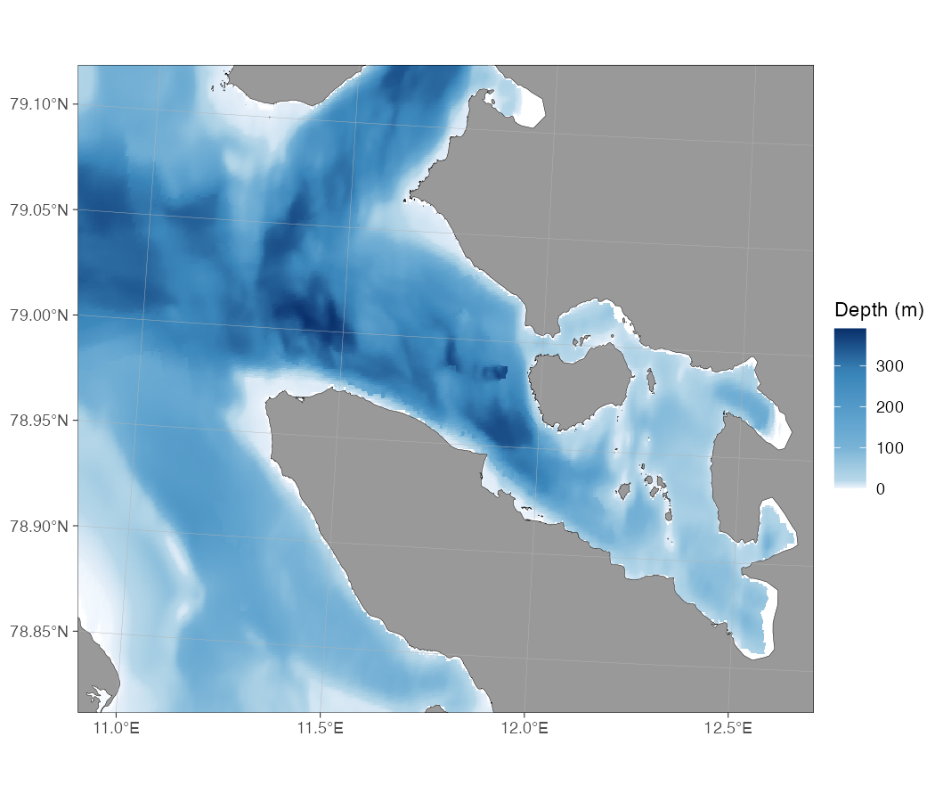
Coupled with the detailed EEA land shapes (shapefiles = "Europe"), this produces the highest-resolution maps ggOceanMaps has generated so far. Being able to plot Norwegian fjords with this level of detail is a significant improvement and has been a popular feature request. With v3, it is possible. Here is Kongsfjorden in Svalbard, drawn over the detailed Svalbard land shapes:

basemap(
  limits = c(10.9, 12.65, 78.83, 79.12),
  bathy.style = "wemb",
  shapefiles = "Svalbard"
)

Figure: Kongsfjorden, Svalbard, with ~115 m EMODnet bathymetry and the detailed Svalbard land shapes.

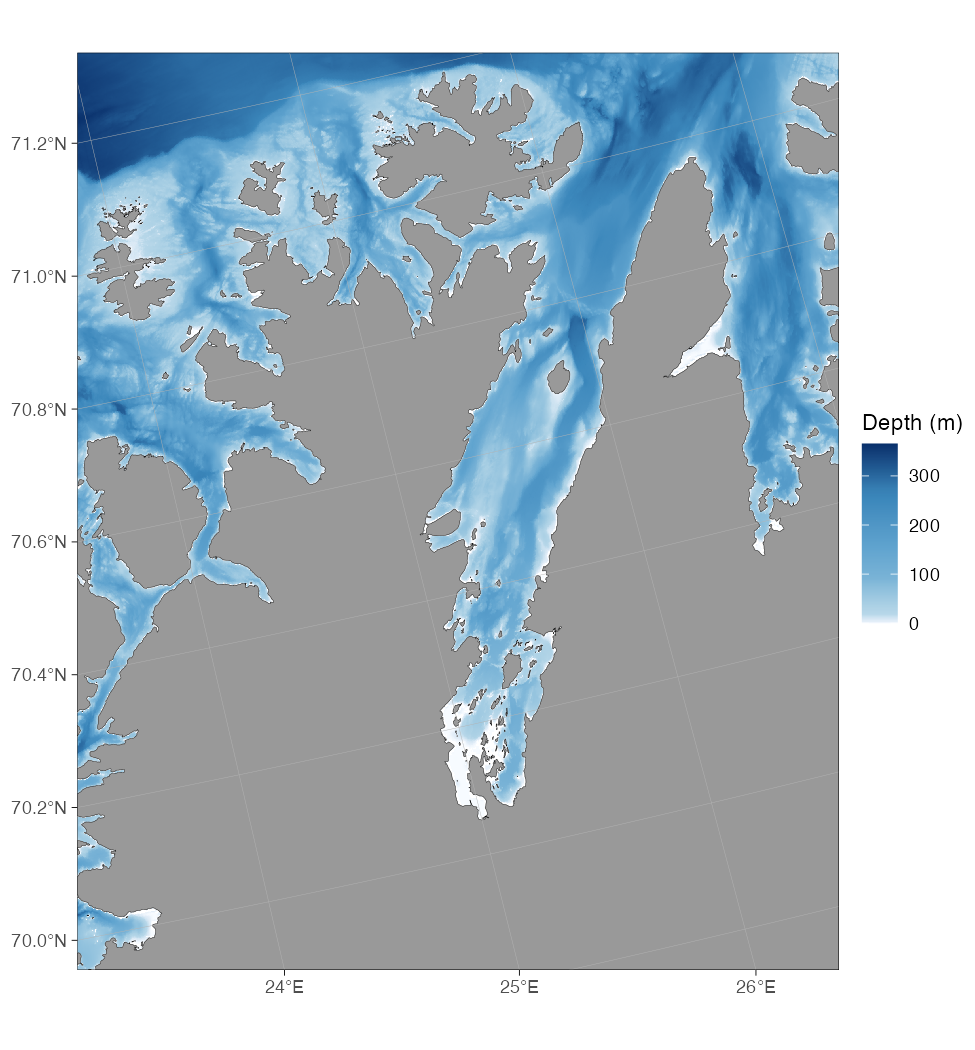
And Porsangerfjorden on the Finnmark coast of mainland Norway, with the EEA "Europe" land shapes:

basemap(
  limits = c(23.9, 26.5, 69.9, 71.15),
  shapefiles = "Europe",
  bathy.style = "wemb"
)

Figure: Porsangerfjorden, northern Norway, with ~115 m EMODnet bathymetry and the EMODnet “Europe” land shapes.

Note that the routine works everywhere in European waters, not just Norway. The downloaded tiles are cached under getOption("ggOceanMaps.datapath"), so re-rendering the exact same map does not re-download anything. Do keep an eye on the size of that folder, though — high-resolution tiles can make it bloat up quickly. Bounding boxes outside a source’s coverage fail cleanly with a pointer to the right alternative, and large areas are tiled and mosaicked automatically. See the Bathymetry article for the full list of sources and more examples.

Build your own shapefiles

The create-your-own-bathymetry workflow is now complete. raster_bathymetry() turns a GEBCO/ETOPO/IBCAO grid into a bathyRaster, and two vectorisers consume it: vector_bathymetry() for depth-contour polygons (as before) and the new vector_land() for a matching land polygon extracted from the same grid.

rb <- raster_bathymetry(
  bathy = "path/to/your/grid.nc",
  depths = c(50, 100, 200, 500, 1000),
  proj.out = 4326,
  boundary = c(-5, 10, 50, 60)
)

basemap(
  limits = c(-5, 10, 50, 60),
  shapefiles = list(
    land = vector_land(rb), # NEW in v3
    glacier = NULL,
    bathy = vector_bathymetry(rb)
  ),
  bathymetry = TRUE
)

Because land and bathymetry come from the same grid, their edges line up. The Customising shapefiles article walks through this pipeline, clip_shapefile(), and reading Norwegian Geonorge depth data with geonorge_bathymetry().

Expanded documentation

Version 3 splits the old single manual into a concise overview plus a set of focused articles:

Bathymetry — every way to get bathymetry into a map, from the shipped low-resolution grid to on-demand WCS and your own rasters.
Customising shapefiles — supplying your own land, glacier, and bathymetry layers.
Adding graphical elements — ocean-current arrows (velocity quivers and schematic “Figure 1” arrows) and pie charts on maps via scatterpie::geom_scatterpie().
Cookbook — short, copy-pasteable recipes.

Testing

Version 3 adds smoke tests based on the historical regression corpus and vdiffr SVG snapshot tests for visual changes. These tests will be expanded in future releases with issues getting solved over time.

Upgrading from version 2

Version 3 is backwards compatible with version 2 map code; existing basemap() and qmap() calls keep working. If you used the older bathymetry styles, see the version 2 release notes and the Bathymetry article for the current bathy.style names.