Bathymetry in ggOceanMaps
Mikko Vihtakari (Institute of Marine Research)
22 June, 2026
Source:vignettes/bathymetry.Rmd
bathymetry.RmdggOceanMaps plots bathymetry from five kinds of data source. They
differ mainly in resolution and in how much setup they require: the
shipped raster works offline with no preparation, while the
higher-resolution options need either an internet connection or a
one-time download. This vignette describes each source and shows the
bathy.style argument that selects it.
The examples that download or fetch data are not evaluated when the vignette is built; the figures shown for them were rendered beforehand.
Quick decision guide
| Need | Source | bathy.style |
|---|---|---|
| Works offline, no setup (default) | Shipped low-resolution raster | "rbb" |
| Higher detail, global and polar maps | ggOceanMapsLargeData continuous raster | "rcb" |
| Filled depth-band contours | ggOceanMapsLargeData polygon contours | "pb" |
| Contour lines only | ggOceanMapsLargeData contour lines | "cb" |
| Anywhere on the globe, ~1.85 km | ETOPO1 Web Coverage Service (live) | "wceb" |
| European waters, ~115 m | EMODnet Web Coverage Service (live) | "wemb" |
| Your own GEBCO / ETOPO / IBCAO file | Local raster via userpath
|
"rub" |
| Custom contour polygons or land |
raster_bathymetry() + vector_bathymetry()
/ vector_land()
|
shapefiles = list(...) |
Substitute g for the final b in any
abbreviation to get the greyscale variant (rbb →
rbg, wemb → wemg, and so on). The
full alias list is in ?basemap.
1. Shipped low-resolution raster (no setup)
The package bundles a coarse global bathymetry raster,
dd_rbathy, which is always available and needs no download.
It is downsampled from the ETOPO 2022 15 arc-second global relief model
(NOAA National Centers for Environmental Information, https://doi.org/10.25921/fd45-gt74) and binned into
depth bands. This is the default source, so it is enough to set
bathymetry = TRUE:
The style can also be set explicitly with
bathy.style = "rbb" (raster, binned, blues):
The greyscale variant is "rbg":
The shipped raster is kept coarse to keep the package within CRAN’s size limit. It is well suited to overview maps and exploratory plots; for publication maps one of the higher-resolution sources below is usually preferable.
2. ggOceanMapsLargeData (one-time download per region)
The companion repository ggOceanMapsLargeData
hosts higher-resolution data for the supported regions (Decimal Degree,
Arctic Stereographic, Antarctic Stereographic, and several pre-made
regional shapefile sets). It provides three styles: a continuous raster,
filled polygon contours, and contour lines. basemap()
downloads what it needs on first use and caches it locally.
One-time setup. Choose a permanent directory so the
files persist between R sessions, and add this line to
~/.Rprofile:
options(ggOceanMaps.datapath = "~/ggOceanMaps_data")On the first call for a region a prompt asks you to confirm the download (roughly 15–100 MB depending on the region). Subsequent calls read from the cache and are immediate.
Continuous raster (rcb)
The recommended high-resolution source for most maps.
downsample = n reduces the rendering cost at the expense of
detail.
basemap(c(11, 16, 67.3, 68.6), bathy.style = "rcb")
basemap(c(11, 16, 67.3, 68.6), bathy.style = "rcb", downsample = 10)
basemap(c(11, 16, 67.3, 68.6), bathy.style = "rcg") # greyscale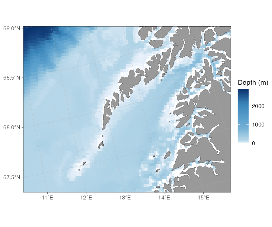
rcb) off Lofoten, northern Norway.Polygon contours (pb)
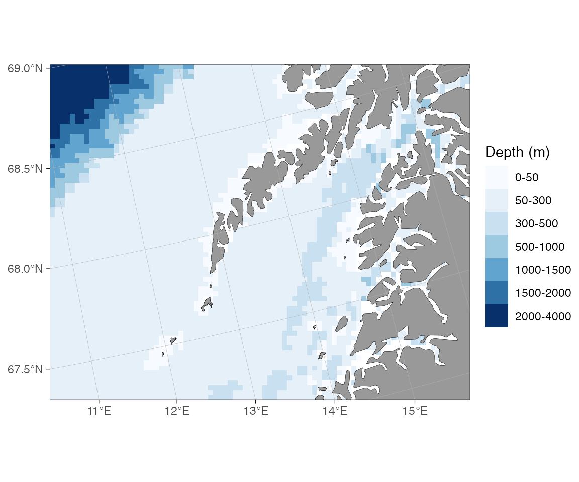
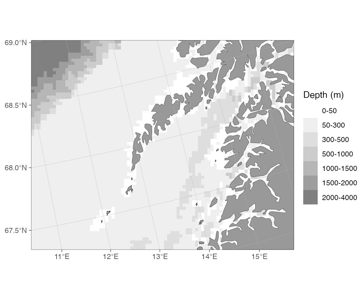
Filled depth bands stored as polygons. This was the default before version 2.0.
basemap(c(11, 16, 67.3, 68.6), bathy.style = "pb")
basemap(c(11, 16, 67.3, 68.6), bathy.style = "pg") # greyscale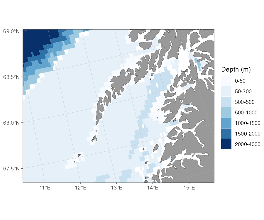
pb) showing filled depth bands.Contour lines (cb)
Depth contours drawn as lines, with no fill. Useful when the bathymetry should not compete visually with overplotted data.
basemap(c(11, 16, 67.3, 68.6), bathy.style = "cb")
basemap(c(11, 16, 67.3, 68.6), bathy.style = "cg") # greyscale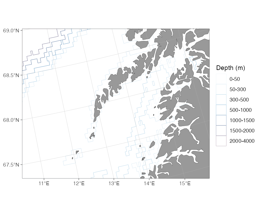
cb), lines only.3. Live download from a Web Coverage Service (WCS)
For one-off maps, or workflows where you would rather not manage
local files, ggOceanMaps can fetch bathymetry on demand from two OGC Web
Coverage Services. No pre-download is required; fetched tiles are cached
under getOption("ggOceanMaps.datapath"), so repeated calls
for the same bounding box are immediate.
| Source | Style | Coverage | Resolution |
|---|---|---|---|
| ETOPO1 (NOAA NCEI) |
wcs_etopo_blues (wceb) |
Global | ~1.85 km |
| EMODnet |
wcs_emodnet_blues (wemb) |
European waters | ~115 m |
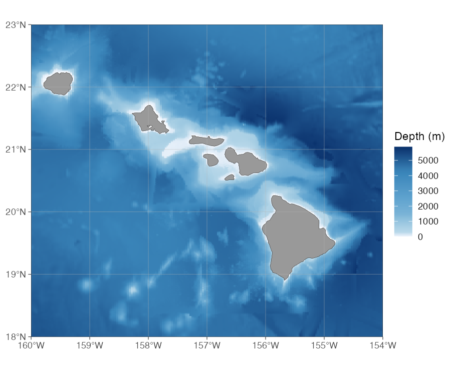
wceb) around the Hawaiian Islands.
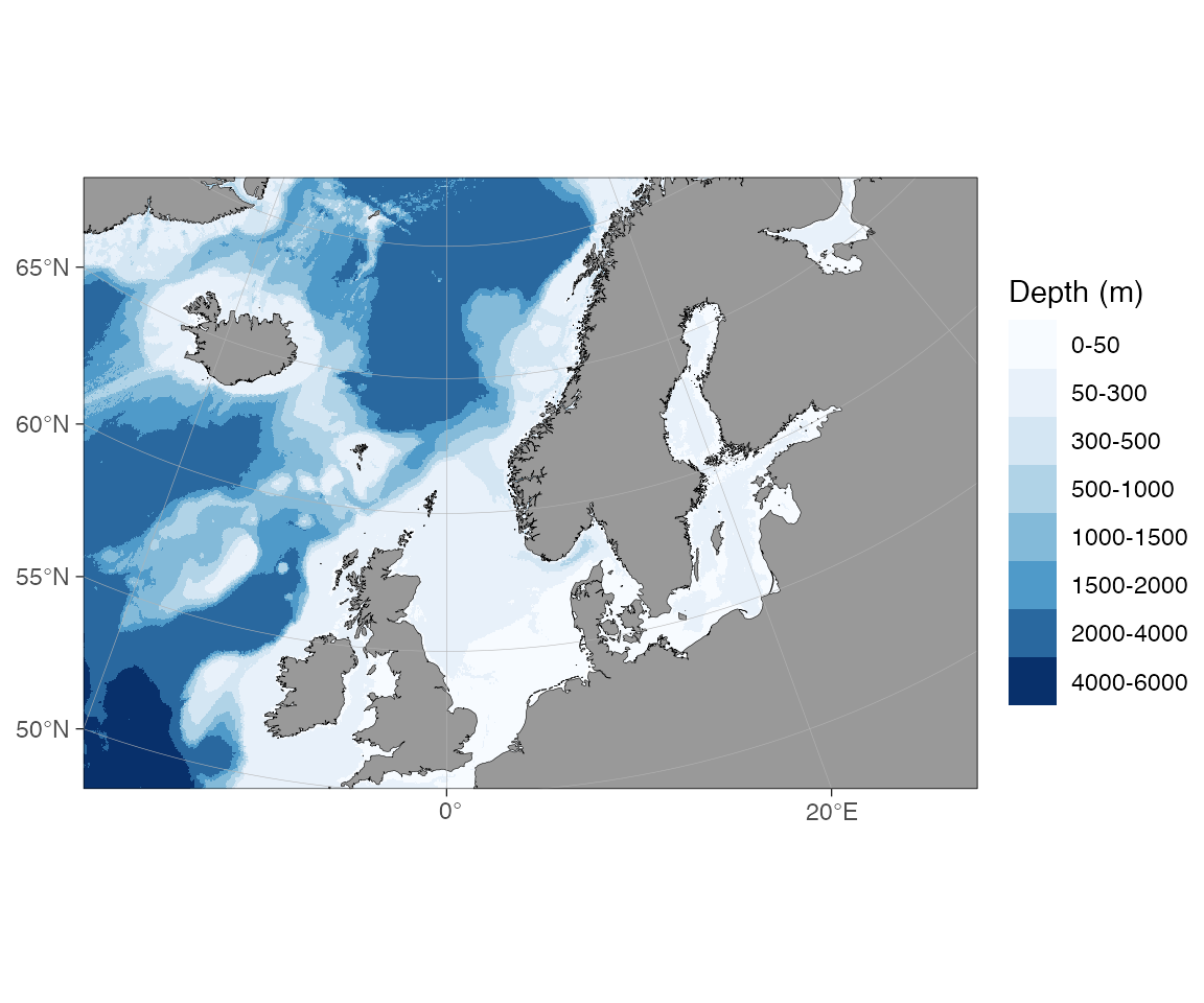
# North Sea — high-resolution European waters from EMODnet
basemap(c(2, 3, 54, 55), bathy.style = "wemb")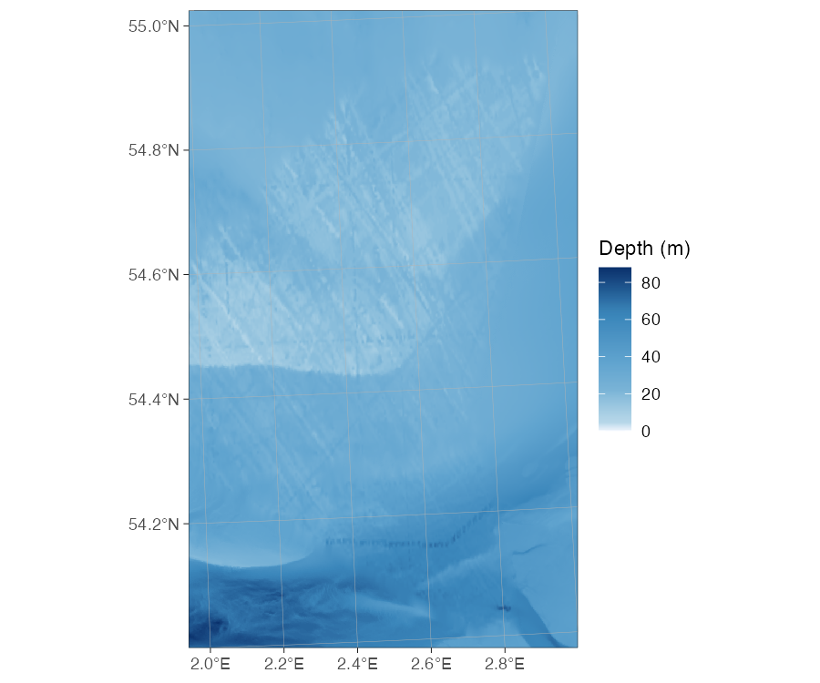
wemb) in the North Sea.If you request EMODnet for an area outside its European coverage, the error message points you to ETOPO:
basemap(c(110, 120, -20, 30), bathy.style = "wemb")
#> Error: Bounding box (110.0° to 120.0° lon, -20.0° to 30.0° lat) lies
#> entirely outside the approximate coverage of EMODnet (≈-36° to 43° lon,
#> 15° to 90° lat).
#> For global bathymetry coverage, download GEBCO or ETOPO data locally and
#> use raster_bathymetry() + vector_bathymetry() instead, or wait for a
#> global WCS source to be added to ggOceanMaps.
Replacing wemb with wceb makes the same
call work.
Manual fetch with wcs_bathymetry()
The bathy.style route is the simplest option, but for
full control — passing the raster into vector_bathymetry(),
combining regions, or sharing a cache with other tools — call
wcs_bathymetry() directly:
bathy <- wcs_bathymetry(c(2, 3, 54, 55), source = "emodnet")

basemap(c(2, 3, 54, 55),
        shapefiles = list(land = dd_land, glacier = NULL,
                          bathy = bathy$raster),
        bathymetry = TRUE)
WCS caveats
- Decimal-degree limits only. Polar maps and projected-CRS limits are not yet supported.
-
Per-source size caps. EMODnet defaults to a 50 deg²
maximum bounding box (it reads 8-byte doubles internally, and a 4° tile
already exceeds its read cap); ETOPO defaults to 2000 deg² because the
underlying grid is much coarser. Override either with
max_area_deg2 = ...inwcs_bathymetry(). Larger boxes are tiled and mosaicked automatically.
4. Your own raster (GEBCO, ETOPO, IBCAO, …)
When you need a specific dataset — the latest GEBCO grid, an ETOPO
2022 variant, a regional IBCAO compilation, or a file processed by your
own group — download it once, point ggOceanMaps at it through
ggOceanMaps.userpath, and use the rub /
rug styles:
# Set once (in .Rprofile for persistence):
options(ggOceanMaps.userpath = "path/to/your/bathymetry.nc")

# Then any basemap call uses your file:
basemap(c(11, 16, 67.3, 68.6), bathy.style = "rub")
basemap(c(11, 16, 67.3, 68.6), bathy.style = "rub", downsample = 10)
basemap(c(11, 16, 67.3, 68.6), bathy.style = "rug") # greyscale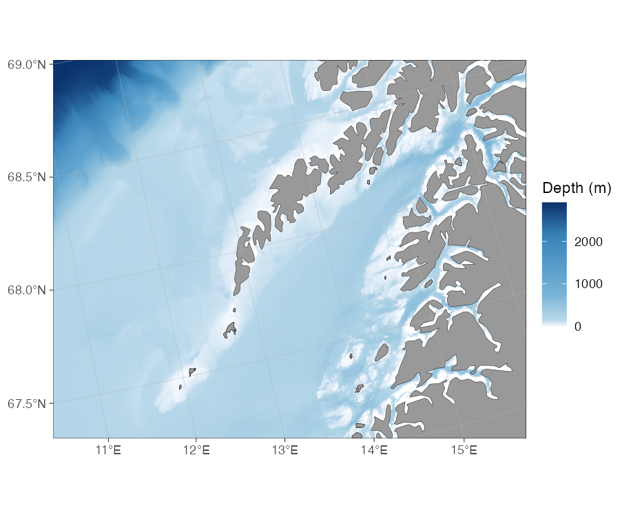
rub) off Lofoten.Any format that stars::read_stars() can open is accepted
(NetCDF .nc, GeoTIFF .tif, GMT
.grd, and so on). The file is read in full on every call,
so the user-raster route can be slower than a pre-processed
ggOceanMapsLargeData object for the same region. Use
downsample to trade resolution for speed.
ggOceanMaps.userpath is also used by
get_depth() to look up point depths from your raster:
dt <- data.frame(lon = seq(-20, 80, length.out = 41), lat = 50:90)
dt <- get_depth(dt, bathy.style = "ru")
qmap(dt, color = depth) + scale_color_viridis_c()
5. Build your own shapefiles
When you need contour polygons, custom depth bins, or a matched land
+ bathymetry pair, the raster_bathymetry() /
vector_bathymetry() / vector_land() pipeline
turns any raster source into reusable shapefile objects:
# 1. Process the raster — crop, sign-flip, optionally bin into contours
rb <- raster_bathymetry(
  "path/to/your/bathymetry.nc",
  depths = c(50, 200, 500, 1000, 2000, 4000),  # depth break points
  boundary = c(-5, 10, 50, 60)                  # crop to your region
)

# 2a. Vectorize bathymetry into depth-band polygons
vb <- vector_bathymetry(rb, drop.crumbs = 10)   # drop islands < 10 km²

# 2b. Vectorize land from the same raster
vl <- vector_land(rb, drop.crumbs = 10)

# 3. Plot — both layers plug into basemap()
basemap(c(-5, 10, 50, 60),
        shapefiles = list(land = vl, glacier = NULL, bathy = vb),
        bathymetry = TRUE)
Setting depths = NULL skips the binning step and returns
a continuous raster — useful for geom_raster-style fills
without the vectorization overhead.
Save the processed objects so the processing cost is paid only once:
save(vb, vl, file = "my_region_bathy.rda")Mixing styles across a multi-panel figure
bathy.style is set per call, so each panel of a
multi-panel figure can use its own source:
Citing the data sources
The bathymetry data are not the property of ggOceanMaps or the Institute of Marine Research. Cite the source of any bathymetry you publish:
-
Shipped raster (
rbb) and ggOceanMapsLargeData rasters / contours (rcb,pb,cb). ETOPO 2022 15 Arc-Second Global Relief Model (NOAA National Centers for Environmental Information, DOI: 10.25921/fd45-gt74). Distributed under the U.S. Government Work license. -
Global Web Coverage Service bathymetry (
wceb/wceg). ETOPO1 Global Relief Model served live by NOAA NCEI (Amante & Eakins 2009, NOAA NGDC, DOI: 10.7289/V5C8276M). Distributed under the U.S. Government Work license. -
European Web Coverage Service bathymetry (
wemb/wemg). EMODnet Bathymetry. Distributed under the CC BY 4.0 license. -
User raster (
rub/rug). Whatever dataset you supplied (GEBCO, ETOPO, IBCAO, …); cite it under its own licence.
The land and glacier polygons, and the regional pre-made shapefiles, have their own sources. See the Citations and data sources section of the README for the full list.
See also
-
?basemapfor the fullbathy.stylereference table. -
?wcs_bathymetryfor the live download function. -
?raster_bathymetry,?vector_bathymetry,?vector_landfor the build-your-own pipeline. - Cookbook for short, copy-pasteable recipes.
- User manual.