ggOceanMaps User Manual

Mikko Vihtakari (Institute of Marine Research)

15 January, 2024

The ggOceanMaps package for R allows plotting data on bathymetric maps using ggplot2. The package is designed for ocean sciences and greatly simplifies bathymetric map plotting anywhere around the globe. ggOceanMaps uses openly available geographic data. Citing the particular data sources is advised by the CC-BY licenses whenever maps from the package are published (see the Citations and data sources section). Note that the package comes with absolutely no warranty and that maps generated by the package are meant for plotting scientific data only. The maps are coarse generalizations of third-party data and therefore inaccurate.

Basic use

ggOceanMaps extends on ggplot2. The package uses spatial (sf) shape- (e.g. vector) and (stars) raster files, geospatial packages for R to manipulate, and ggplot2 to plot these data. The vector and raster plotting is conducted internally in the basemap function, which uses ggplot’s sf object plotting capabilities.

The primary aim of ggOceanMaps is to make plotting oceanographic spatial data as simple as feasible, but also flexible for custom modifications. The “as simple as feasible” part will be covered in this section, while the “flexible for custom modifications” part is covered in the Advanced use section. The basic use section of this tutorial assumes that the user knows how to use ggplot2. If you are not familiar with this package, you may read the Data visualization section in Hadley Wickham & Garrett Grolemund. This tutorial does not describe functions in ggOceanMaps but rather focuses on how to use them. Make sure to refer to the function documentation while reading the tutorial.

library(ggOceanMaps)

Limiting maps

To ensure simplicity, ggOceanMaps package attempts to use decimal degree coordinate system as much as possible. This system represents coordinates on a sphere, while maps are plotted in two dimensions. Therefore, the underlying map data have to be projected using different mathematical algorithms depending on the geographic location.

Maps can be limited (e.g. provide geographic location for a map) using three arguments: limits, data, and shapefiles. The limit type is automatically detected when supplied to the first argument (called x) in the basemap() and qmap() functions.

Limits

The simplest way of defining the geographic location is to use the limits argument with decimal degrees. The limits argument can be defined either as a numeric vector of length 1 or 4. Specifying the argument as a single integer between 30 and 88 or -88 and -30 plots a polar stereographic map for the Arctic or Antarctic, respectively.

library(ggOceanMaps)
library(ggspatial) # for data plotting
basemap(limits = 60) # A synonym: basemap(60)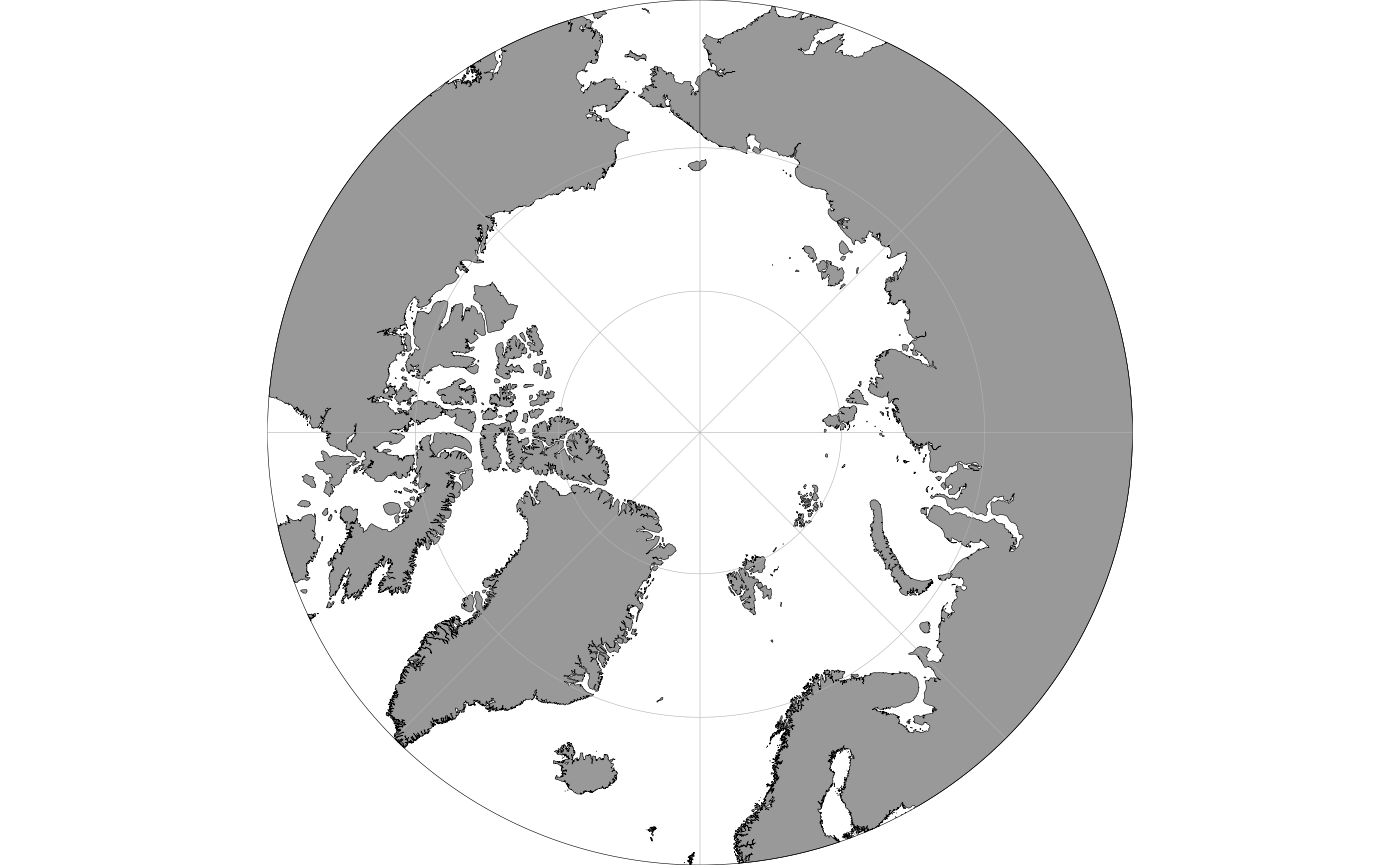 

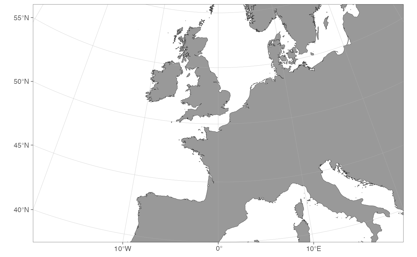
Rectangular maps are plotted by specifying the limits argument as a numeric vector of length 4 where the first element defines the start longitude, the second element the end longitude, the third element the minimum latitude and the fourth element the maximum latitude of the bounding box:

basemap(limits = c(-20, 20, 40, 59))

Limiting maps using decimal degrees is somewhat counter-intuitive because maps plotted for polar regions (>= 60 or <= -60 latitude) are actually projected to Arctic and Antarctic polar stereographic systems. Because decimal degrees are angular units running counter-clockwise, also the longitude limits have to be defined counter-clockwise. Projected maps with decimal degree limits will lead to expanded limits towards the poles when using Arctic and Antarctic Polar Stereographic projections because decimal degrees represent a sphere:

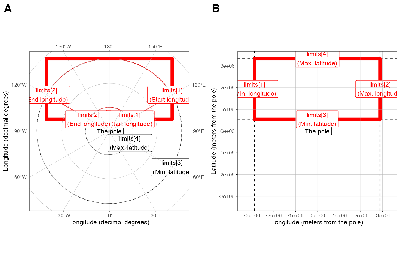
The figure above: Limiting rectangular basemaps is done by placing four coordinates to the limit argument. A) If the limits are in decimal degrees, the longitude limits ([1:2]) specify the start and end segments of corresponding angular lines that should reside inside the map area. The longitude limits are defined counter-clockwise. The latitude limits [3:4] define the parallels that should reside inside the limited region given the longitude segments. Note that the resulting limited region (polygon with thick red borders) becomes wider than the polygon defined by the coordinates (thin red borders). The example limits are c(120, -120, 60, 80). B) If the limits are given as projected coordinates or as decimal degrees for maps with |latitude| < 60, limits elements represent lines encompassing the map area in cartesian space. The example limits are the limits from A) projected to the Arctic stereographic (crs = 3995).

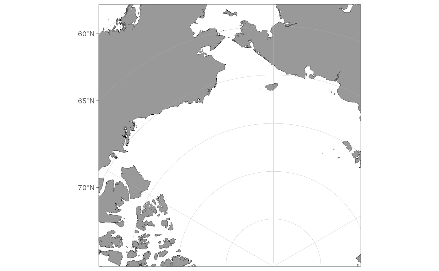
The example above as a map. Note how the latitude limits give a much larger map than one would expect from cartesian coordinates because the 60 \(^\circ\)N parallel is within the map area between 120 \(^\circ\)E and 120 \(^\circ\)W meridians.

dt <- data.frame(lon = c(120, 120, -120, -120), lat = c(60, 80, 80, 60))

basemap(limits = c(120, -120, 60, 80)) +
  ggspatial::geom_spatial_polygon(
    data = dt, 
    aes(x = lon, y = lat), fill = NA, color = "red")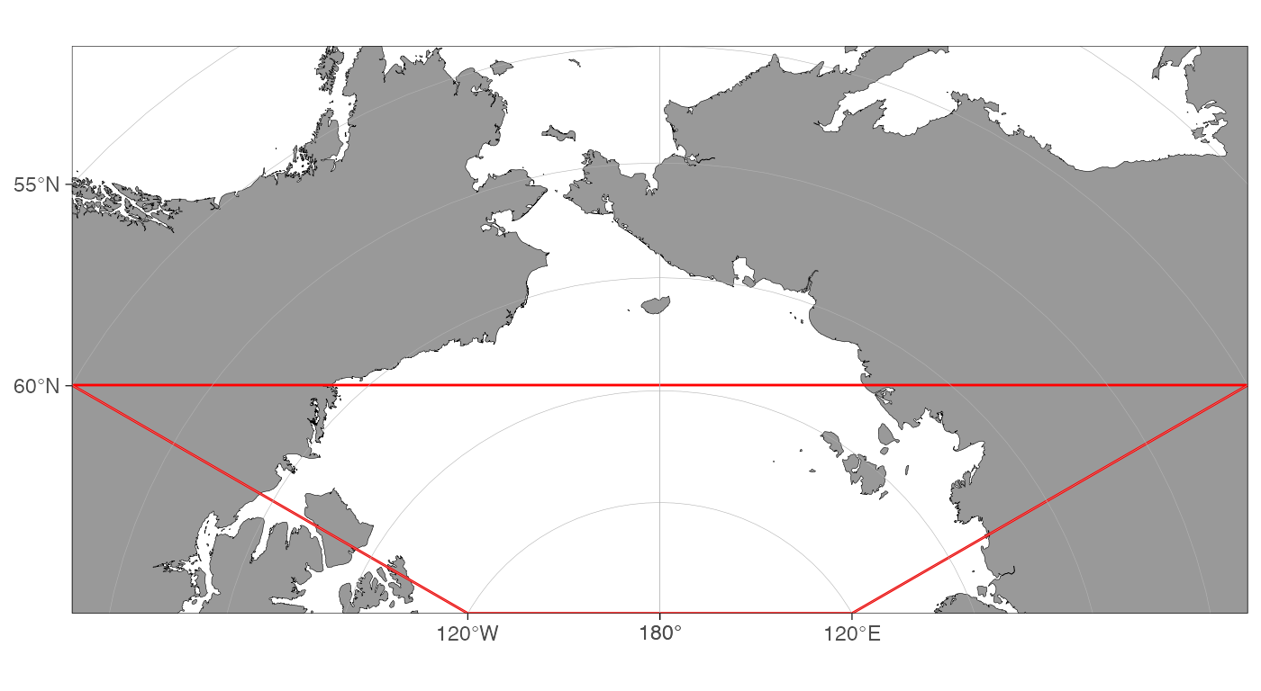

Exact control of map limits can be difficult using decimal degree limits in polar regions. The limits argument also allows specifying the limits in the underlying projected coordinate units. First, we will need to find out how these units look like:

basemap(limits = 60, projection.grid = TRUE, grid.col = "red")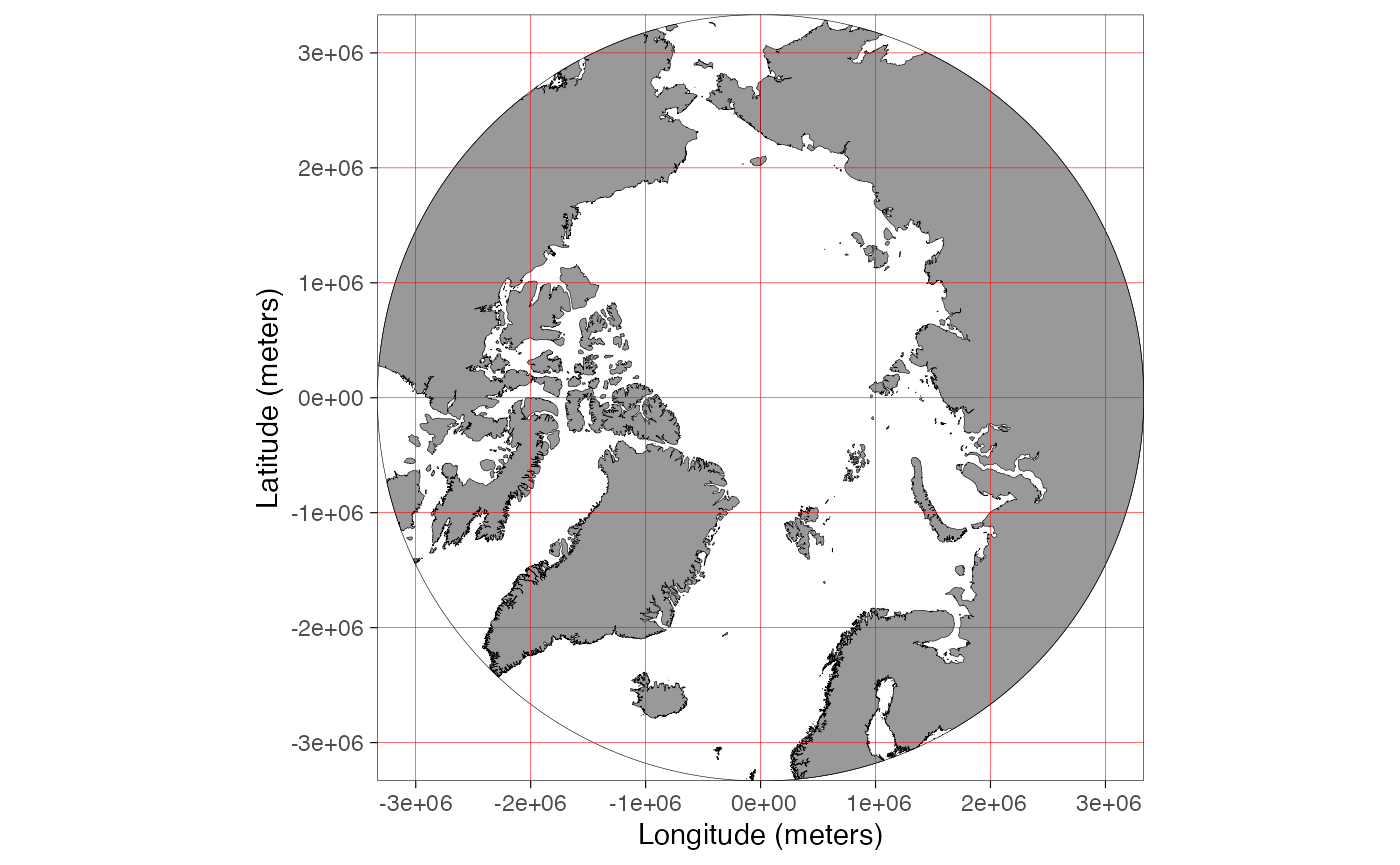

The projection.grid argument plots a grid using the projected actual map coordinates instead of decimal degrees. The grid helps in defining the limits using projected coordinates giving better control over the map limits than decimal degree coordinates. The automatic shapefile definition algorithm does not work for projected coordinates. Therefore, if the limits are not given as decimal degrees (any longitude outside the range [-180, 180] or latitude [-90, 90]), the function asks to specify shapefiles. The shapefiles can be defined by partially matching the names of the pre-made shapefiles in shapefile_list (e.g. “Ar” would be enough for “ArcticStereographic”):

basemap(limits = c(-2e6, 1e6, 0, 3e6), shapefiles = "Arctic") 

Data limits

The limits of a map can also be defined by inputting a data frame to the data argument. The limits are automatically defined allowing the user to quickly find limits for a desired spatial dataset:

dt <- expand.grid(lon = c(160, 180, -160), lat = c(60, 70, 80))

basemap(data = dt) + # a synonym: basemap(dt)
  ggspatial::geom_spatial_point(data = dt, aes(x = lon, y = lat), color = "red")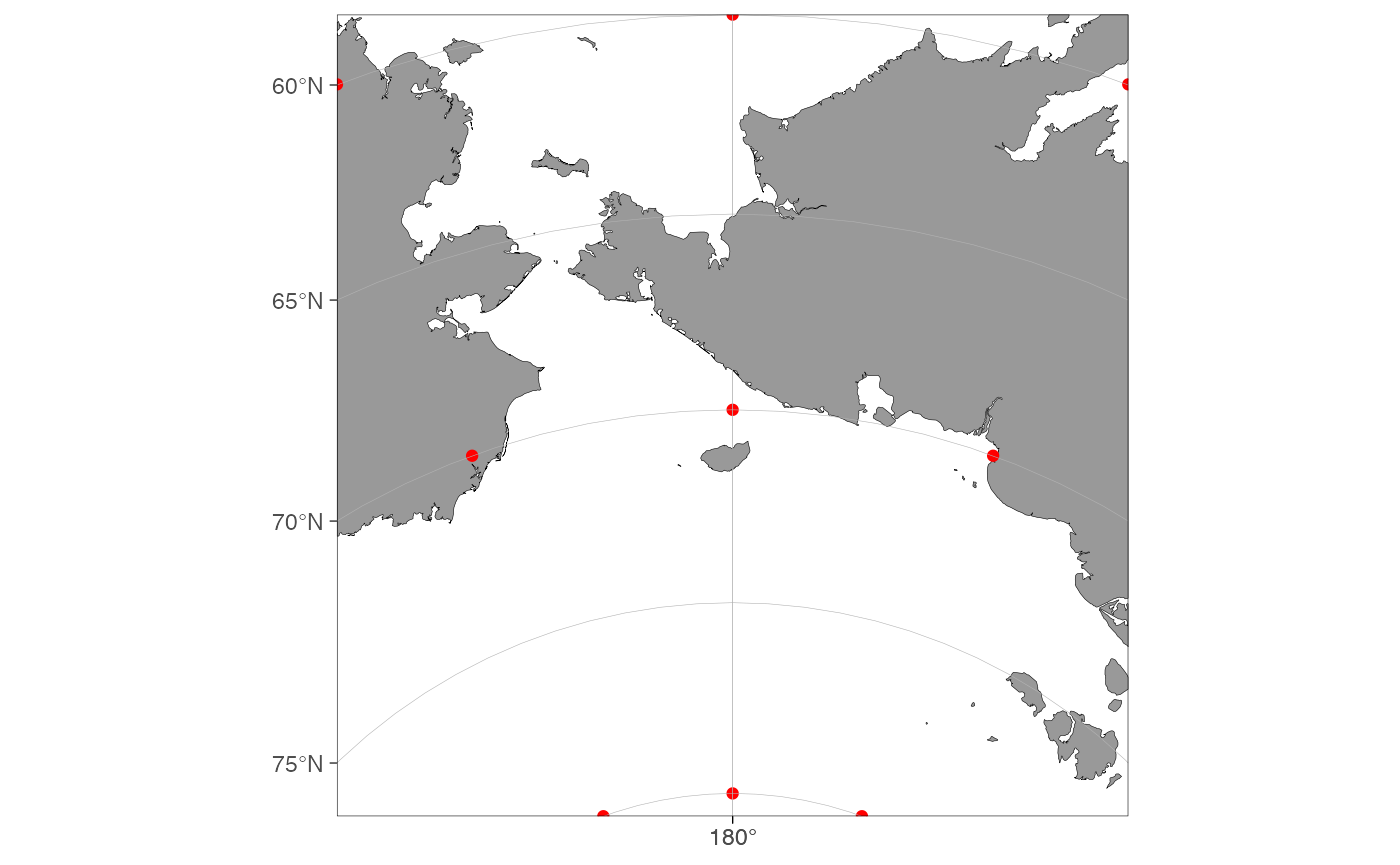

The function makes the map such that the outermost data points barely fit into the mapped region. The space between the map borders and data points can be adjusted using the expand.factor argument:

cowplot::plot_grid(
  basemap(dt, expand.factor = 1.1) +
    ggspatial::geom_spatial_point(data = dt, aes(x = lon, y = lat), color = "red") +
    theme(axis.title = element_blank()),
  basemap(dt, expand.factor = 0.9) +
    ggspatial::geom_spatial_point(data = dt, aes(x = lon, y = lat), color = "red") +
    theme(axis.title = element_blank()),
  labels = "AUTO"
)

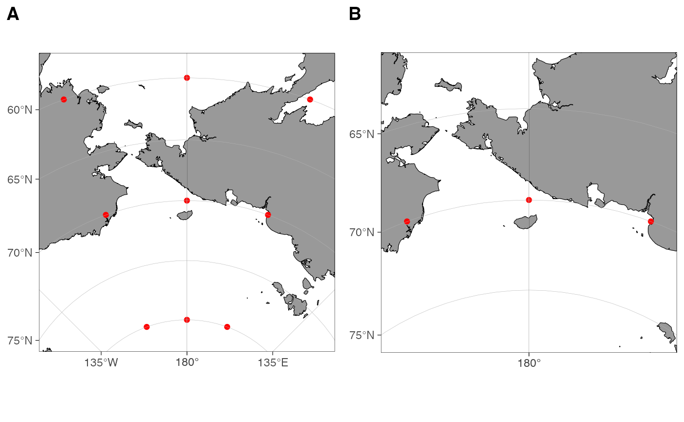
Figure above: The expand.factor argument can be used to expand (A) and reduce (B) map region in relation to data.

See the Adding data to maps section for more information. The basemap() function automatically detects columns containing longitude and latitude information when the data argument is used. The automatic detection algorithm is not very advanced and it is recommended to use intuitive column names for longitude (such as “lon”, “long”, or “longitude”) and latitude (“lat”, “latitude”) columns. The coordinate data have to be given as decimal degrees for the data argument to function.

Shape files

The ggOceanMaps package contains a set of [premade shapefiles]. Only the decimal degree land shapes are shipped with the package while others are downloaded as needed. See the front page for instructions how to setup the automatic download folder before you start downloading shape files. Any character supplied to the x argument in the basemap() function will automatically be understood as shapefiles argument. The maps are limited showing the entire land shape. Use the limits argument to further limit the shape file.

basemap("Arctic")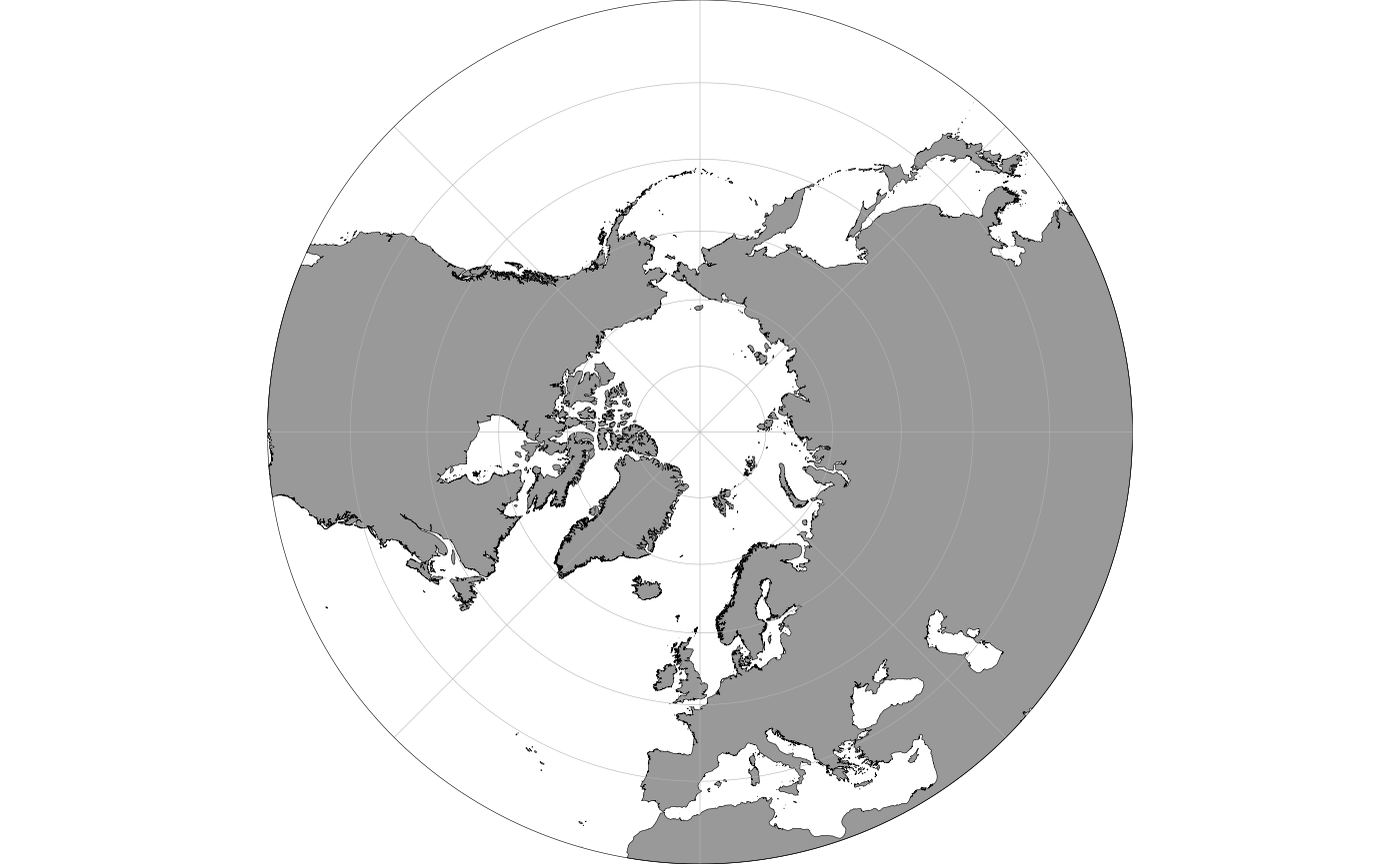

Bathymetry

Bathymetry system was revised in version 2.0. Bathymetry can be plotted by simply specifying bathymetry = TRUE or bathy.style (no need to specify both any longer):

basemap(limits = c(-125, -110, 25, 35), bathymetry = TRUE)

The default, bathy.style = "raster_binned_blues", uses a low-resolution raster file shipped with ggOceanMaps. The package contains an option to plot higher resolution bathymetries than the default binned blue alternative. These bathymetries can be accessed by specifying the bathy.style argument and require a download from ggOceanMapsLargeData or other online repositories.

basemap(limits = c(-125, -110, 25, 35), bathy.style = "rcb") # synonym to "raster_continuous_blues"

The bathy.style character argument consists of three parts separated by a _. The first part gives the type: raster, poly(gon), or contour. The two latter ones use vector data. The second part gives the resolution: binned, continuous or user. The continuous and user options cannot be used for vector data.

The user option accepts any raster file that can be opened using stars::read_stars. The path to the file has to be stored in ggOceanMaps.userpath option (e.g. options(ggOceanMaps.userpath = "PATH_TO_THE_FILE")) (you can set this in .Rprofile to avoid having to type it every time).

The last part defines the color: blues or grays. These options can be abbreviated by specifying the first letter of each part. Gray contour lines are an exception to the rule above and can be plotted using bathy.style = “contour_gray”. Future versions may contain a combination of raster and gray contours, but these have not been implemented yet. Currently implemented bathy.style alternatives are:

• NULL (default). Bathymetry style is searched from getOption("ggOceanMaps.bathy.style"). If not found, "raster_binned_blues" is used.

basemap(c(11,16,67.3,68.6), bathymetry = TRUE)

• "raster_binned_blues" or "rbb" plots binned raster bathymetry filled with different shades of blue. Does not require a download.

basemap(c(11,16,67.3,68.6), bathy.style = "rbb")

• "raster_binned_grays" or "rbg" the same than above but uses different shades of gray.

basemap(c(11,16,67.3,68.6), bathy.style = "rbg")

• "raster_continuous_blues" or "rcb" plots continuous raster bathymetry filled with different shades of blue. More detailed and visually more appealing than the binned bathymetry. Requires a download.

basemap(c(11,16,67.3,68.6), bathy.style = "rcb")

• "raster_continuous_grays" or "rcg" the same than above but uses different shades of gray.

basemap(c(11,16,67.3,68.6), bathy.style = "rcg")

• "raster_user_blues" or "rub" plots continuous raster bathymetry filled with different shades of blue from getOption("ggOceanMaps.user.path"). Any file supported by stars::read_stars should work. The file has to be placed into the location specified by the path. Experimental feature. Has been tested using ETOPO 60 arc-second and GEBCO 15 arc-second grids. Please report any bugs you find.

basemap(c(11,16,67.3,68.6), bathy.style = "rub")

• "raster_user_grays" or "rug" the same than above but uses different shades of gray.

basemap(c(11,16,67.3,68.6), bathy.style = "rug")

• "poly_binned_blues", "poly_blues", "pbb" and "pb" plot polygon bathymetry filled with different shades of blue. Default in the versions older than 2.0 of ggOceanMaps. Requires a download.

basemap(c(11,16,67.3,68.6), bathy.style = "pb")

• "poly_binned_grays", "poly_grays", "pbg" or "pg" same than above but uses different shades of gray.

basemap(c(11,16,67.3,68.6), bathy.style = "pg")

• "contour_binned_blues", "contour_blues", "cbb" or "cb" contour lines with different shades of blue. Requires a download.

basemap(c(11,16,67.3,68.6), bathy.style = "cb")

• "contour_gray", "contour_gray" or "cg" plots gray contour lines. Requires a download.

basemap(c(11,16,67.3,68.6), bathy.style = "cg")

The default bythy.style can be changed by setting the ggOceanMaps.bathy.style option. options(ggOceanMaps.bathy.style = "poly_blues") would make the style similar to older pre-2.0 versions of ggOceanMaps.

Glaciers

Since 2.0, glaciers require a download. It is a good idea to use the polar stereographic datasets for this purpose:

basemap(limits = -60, glaciers = TRUE, shapefiles = "Antarctic")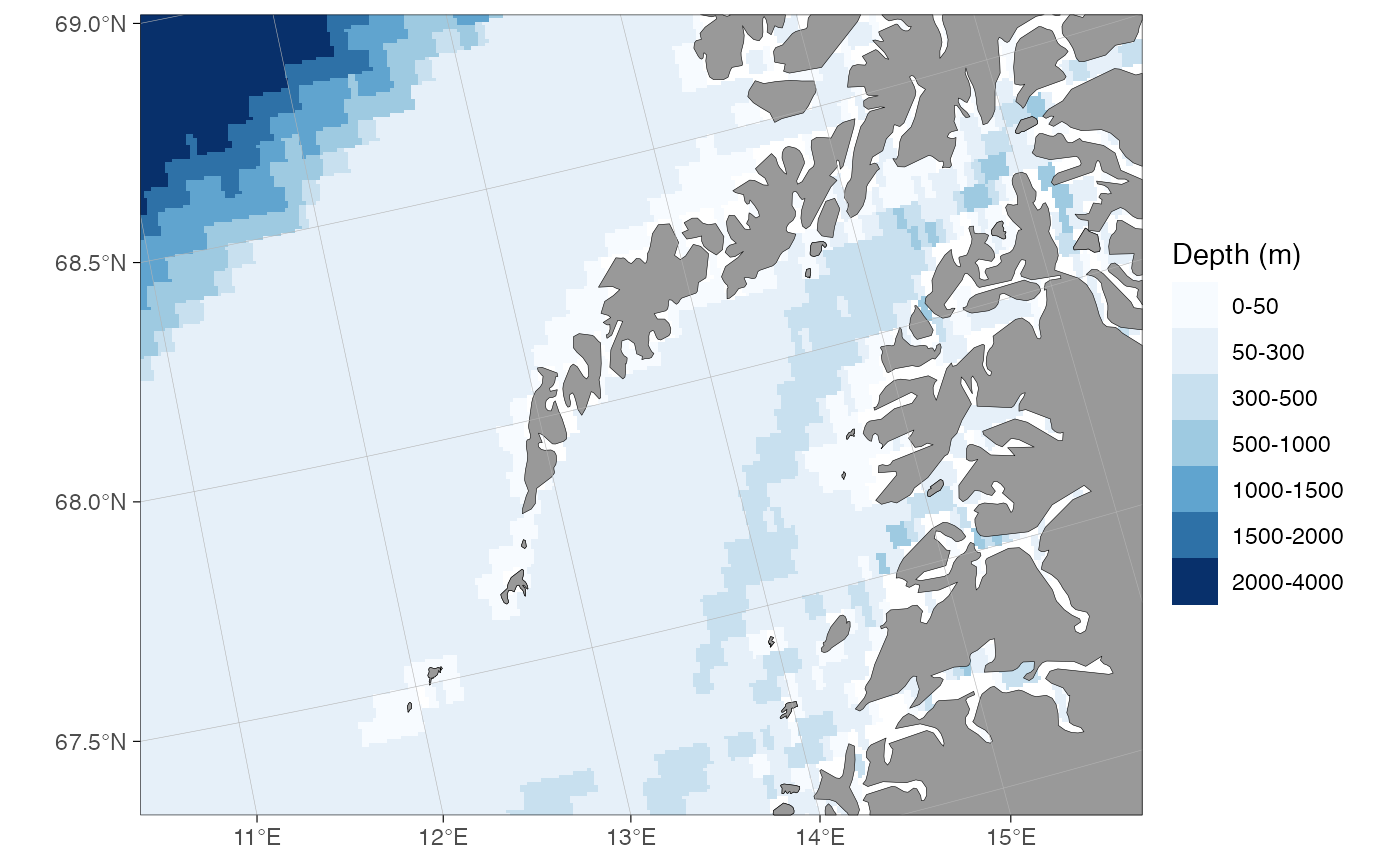

Adding data to maps

The basemap(...) function works almost similarly to the ggplot(...) function as a base for adding further layers to the plot. The difference between the basemap() and the ggplot() is that the basemap() plot already contains multiple ggplot layers. All layers except bathymetry have no other aes mapping than x, y and group. Bathymetry is mapped to fill or color color in addition. This means that when you add ggplot layers, you need to specify the data argument explicitly as shown below. Another difference is that basemaps are plotted using projected coordinates. The ggspatial and ggplot’s geom_sf functions convert the coordinates automatically to the projected coordinates:

dt <- data.frame(lon = c(seq(-180, 0, 30), seq(30, 180, 30)), lat = -70)

basemap(limits = -60, glaciers = TRUE, shapefiles = "Antarctic") + 
  ggspatial::geom_spatial_point(data = dt, aes(x = lon, y = lat), color = "red")

The ggplot functions can also be used, but the coordinates need to be transformed to the basemap projection first using the transform_coord function:

basemap(limits = -60, glaciers = TRUE, shapefiles = "Antarctic") + 
  geom_point(data = transform_coord(dt), aes(x = lon, y = lat), color = "red")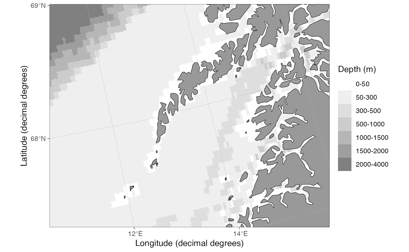

Note that the maps plotted in temperate and tropical regions are not projected. Consequently, decimal degrees work for such maps directly:

dt <- data.frame(lon = c(-100, -80, -60), 
                 lat = c(10, 25, 40), 
                 var = c("a", "a", "b")
)

basemap(data = dt) + 
  geom_point(data = dt, aes(x = lon, y = lat), color = "red")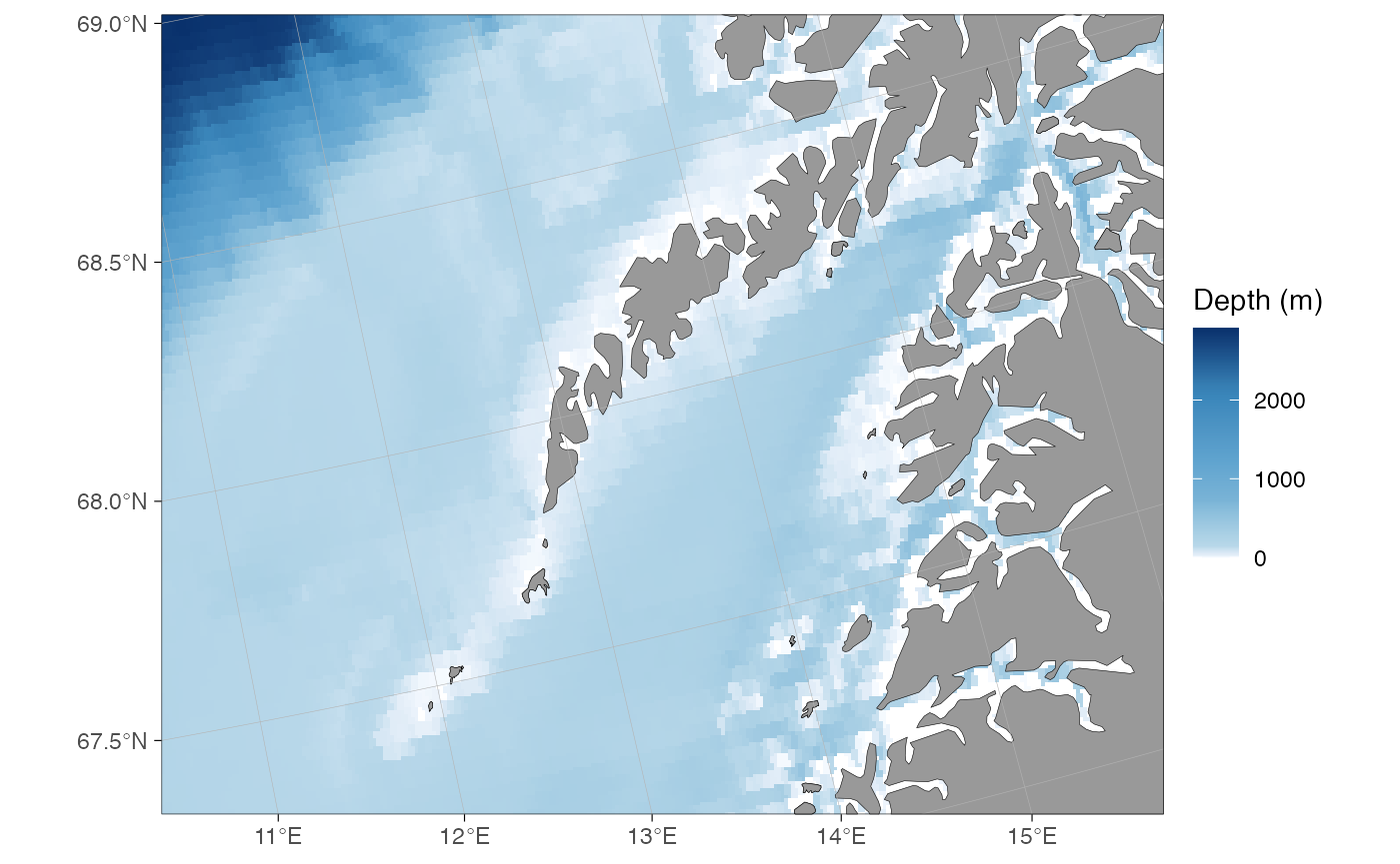

The transform_coord function detects the projection automatically, given that the map is limited using a similar range of coordinates. Therefore you can use the transform_coord as demonstrated above whenever using standard ggplot layers.

transform_coord(data.frame(lon = -80, lat = 25), bind = TRUE)

#>   lon lat lon.proj lat.proj
#> 1 -80  25      -80       25

Rotating maps

The stereographic maps can be rotated to point towards north using the rotate argument:

basemap(limits = c(-160, -80, 60, 85), rotate = TRUE)

Note that rotation changes the underlying CRS and data need to be added using ggspatial::geom_spatial_*, ggplot2::geom_sf() or transform_coord(rotate = TRUE) functions.

Quick map

The qmap function is designed as a shortcut to quickly take a look at a spatial dataset. This function automatically detects the type of data fed into the function and plots a map using appropriate geometries, limits, and projection. You can use the expand.factor argument to adjust the automatic zoom into data.

dt <- data.frame(lon = c(-100, -80, -60), 
                 lat = c(10, 25, 40), 
                 var = c("a", "a", "b")
)

qmap(dt, color = I("red")) # set color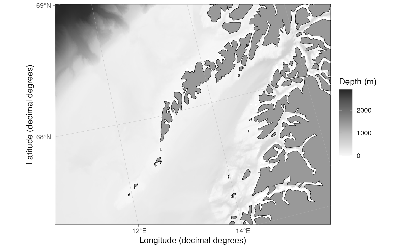

qmap(dt, color = var, expand.factor = 1.3) # map color, zoom out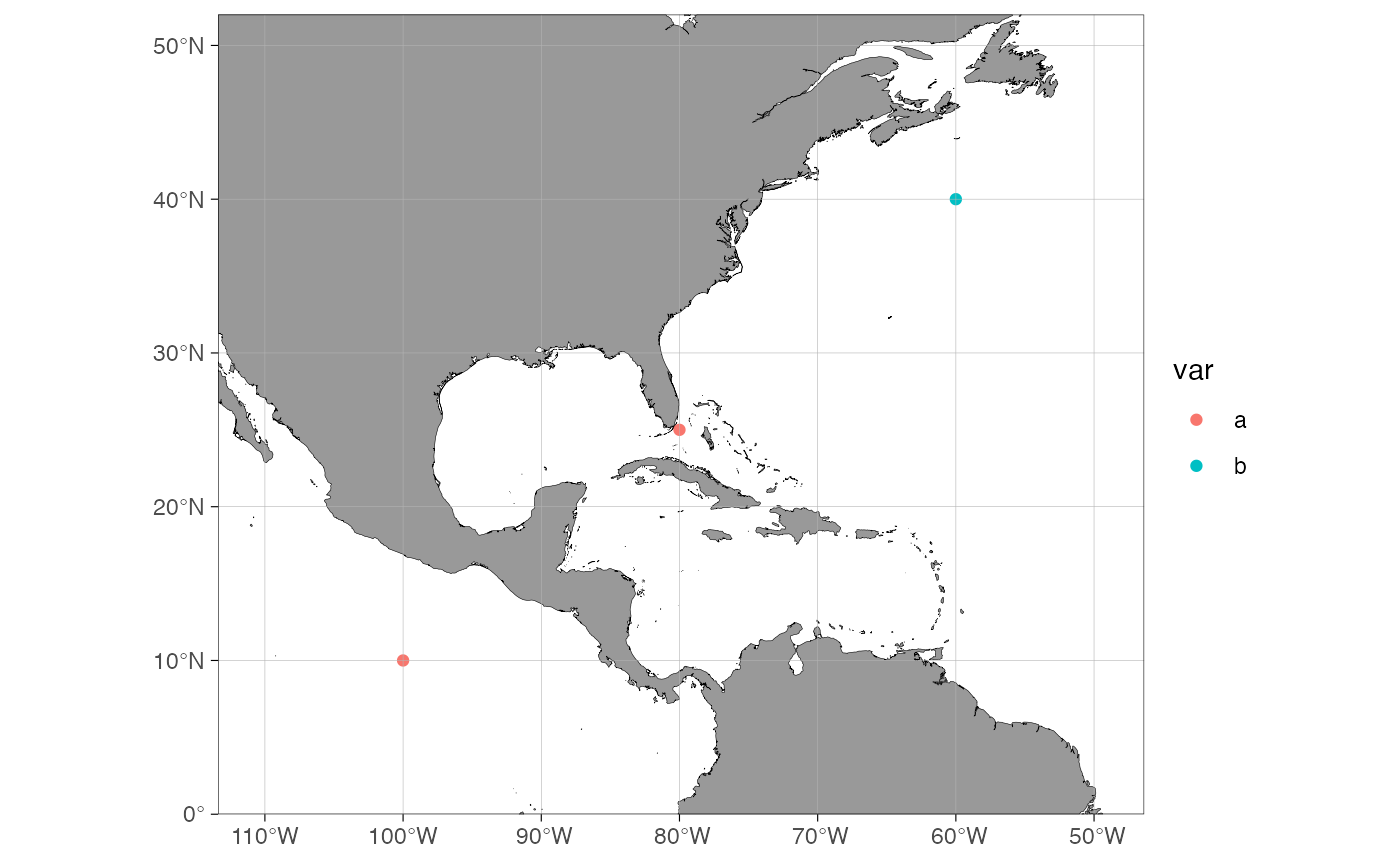

Advanced use

This section focuses on flexibility and user modifications. It is assumed that advanced users understand the basics of geographic information systems (GIS) and how to use these systems in R (e.g. see the Making Maps with R chapter in Lovelace et al. 2020).

Projections

The basemap function uses the limits argument to automatically detect the required projection for a map (or the data argument to calculate limits). The algorithms deciding which projection to use are defined in define_shapefiles and shapefile_list functions. The basemap function uses decimal degree land shapes as default and transforms them to polar stereographic projections based on following rules (given as EPSG codes):

• 4326 WGS 84 / World Geodetic System 1984, used in GPS. Called “DecimalDegree”. For min latitude (limits[3]) < 30 or > -30, max latitude (limits[4]) < 60 or > -60, and single integer latitudes < 30 and > -30.
• 3995 WGS 84 / Arctic Polar Stereographic. Called “ArcticStereographic”. For max latitude (limits[4]) >= 60 (if min latitude (limits[3]) >= 30), and single integer latitudes >= 30 and <= 89.
• 3031 WGS 84 / Antarctic Polar Stereographic. Called “AntarcticStereographic”. For max latitude (limits[4]) <= -60 (if min latitude (limits[3]) <= -30), and single integer latitudes <= -30 and >= -89.

Further, there are higher resolution data that can be downloaded when needed. They use a projection which suits that region. Here are all shapefiles and their projections (CRS):

name	crs
ArcticStereographic	3995
AntarcticStereographic	3031
DecimalDegree	4326
Svalbard	32633
Europe	3035

Since 2.0, it is possible to override the default CRS used by basemap() using the crs argument:

basemap(limits = c(0, 15, 55, 65), crs = 32631)

Appearance

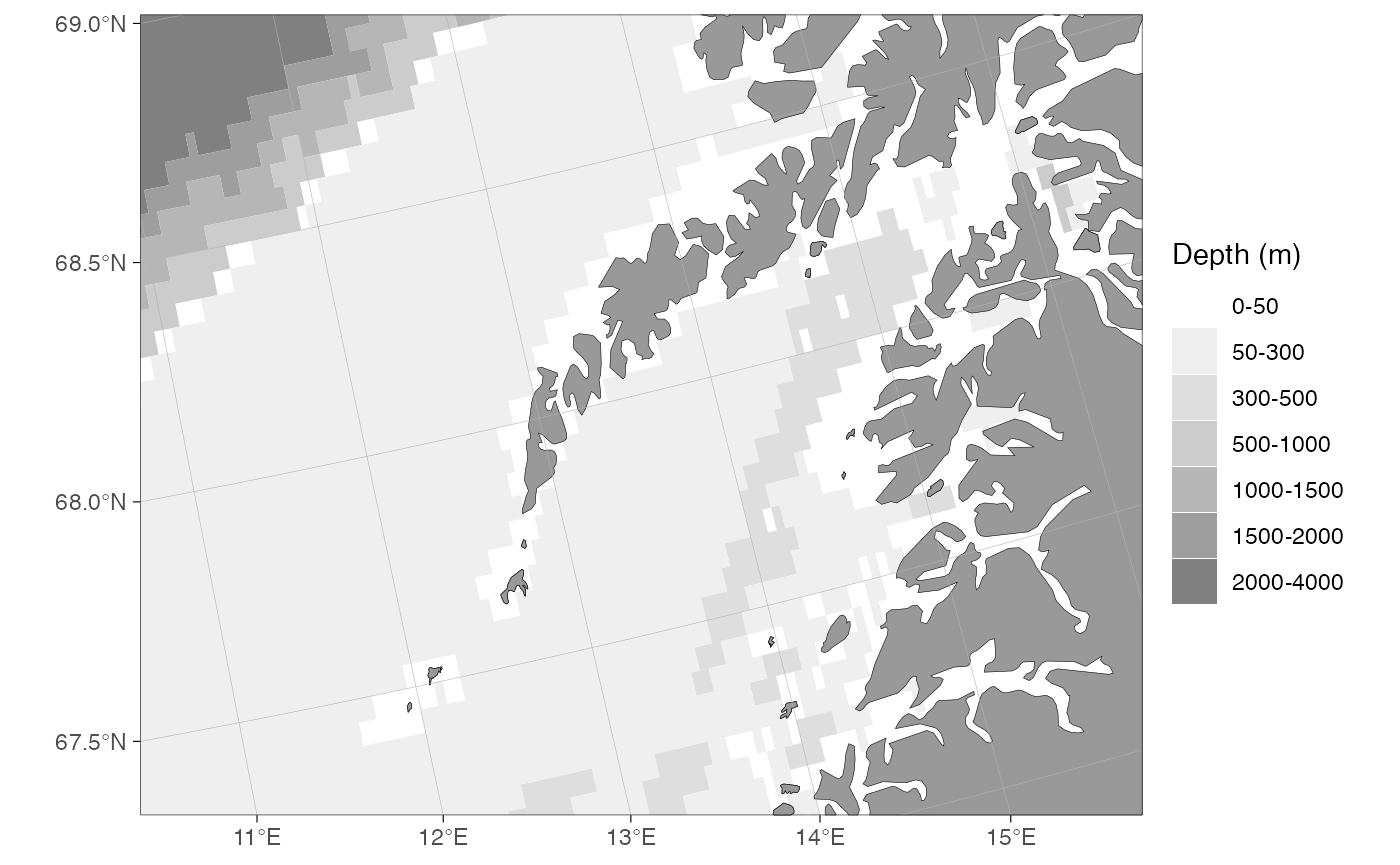
Customizing bathymetry scales

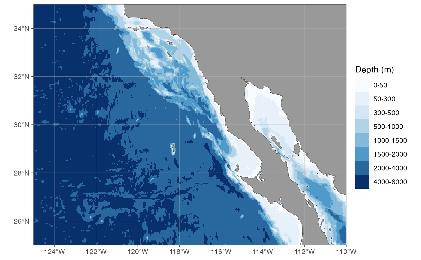
The bathy.style = "*_binned_*" bathymetry polygons are mapped to geom_fill_discrete and can be modified using standard ggplot syntax:

basemap(limits = c(-140, -105, 20, 40), bathymetry = TRUE) + 
  scale_fill_viridis_d("Water depth (m)")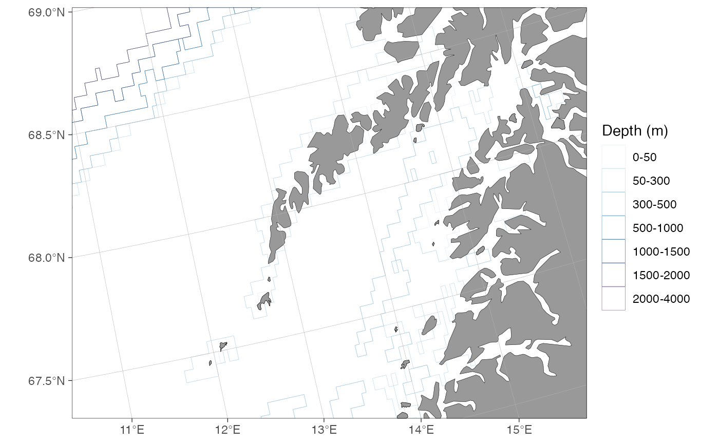

The bathy.style = "*_continuous_*" bathymetry polygons are mapped to geom_fill_continuous:

basemap(limits = c(-140, -105, 20, 40), bathy.style = "rcb") + 
  scale_fill_viridis_c("Water depth (m)")

The bathy.style = "contour_*" bathymetry lines are mapped to geom_color_discrete:

basemap(limits = c(0, 60, 68, 80), bathymetry = TRUE, bathy.style = "contour_blues") + 
  scale_color_hue()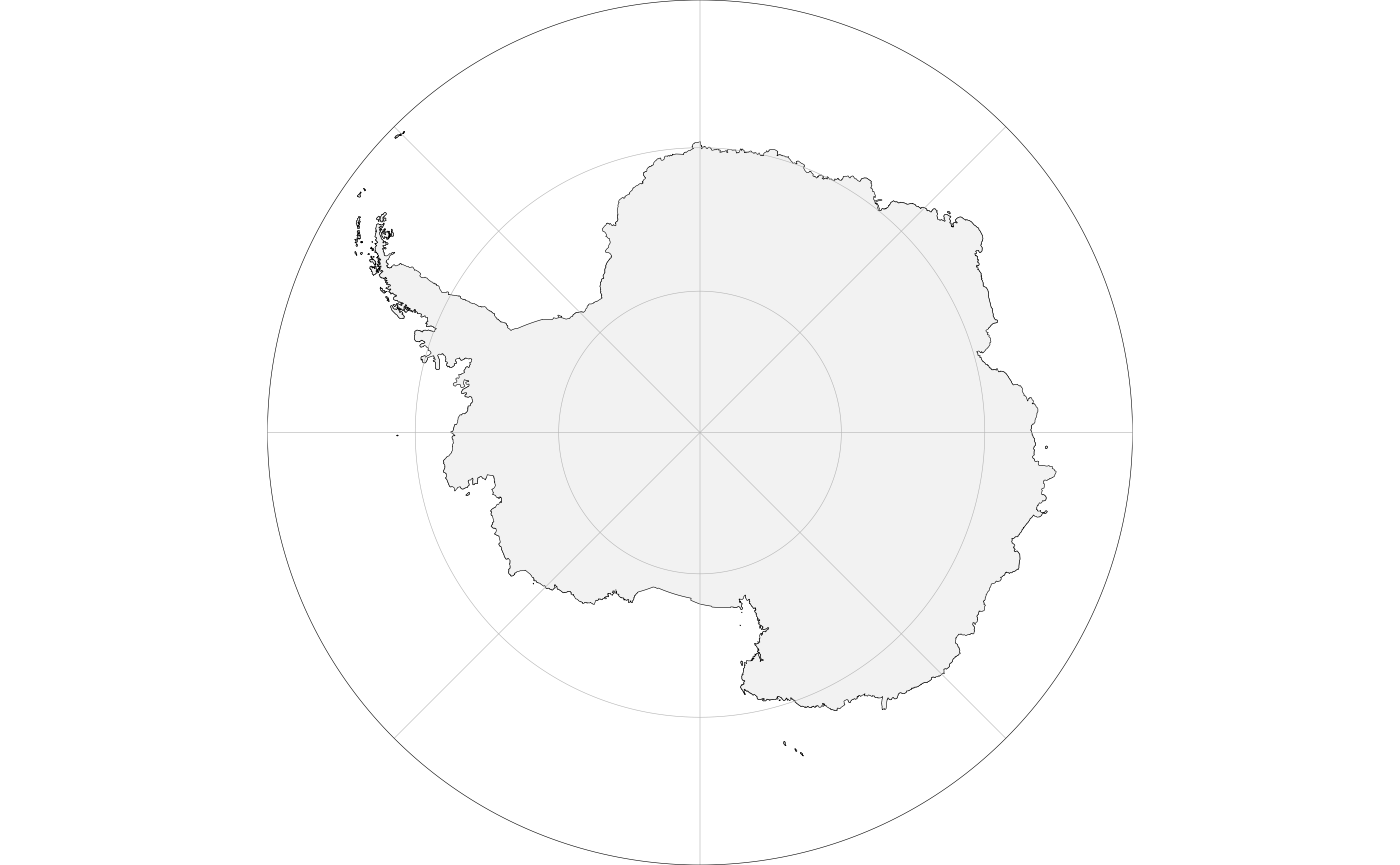

Graphical parameters

The basemap function uses graphical parameters that (very objectively) happen to please the eye of the author and have worked in the applications needed by the author. The default parameters may suddenly change without warning. You may want to modify the appearances of a basemap to your own liking. This can be done using the *.col (fill), *.border.col (line color) and *.size (line width) arguments:

basemap(limits = c(-20, 30, 55, 70), glaciers = TRUE, 
        bathymetry = TRUE, bathy.style = "poly_greys",
        land.col = "#eeeac4", gla.col = "cadetblue", 
        land.border.col = NA, gla.border.col = NA,
        grid.size = 0.05)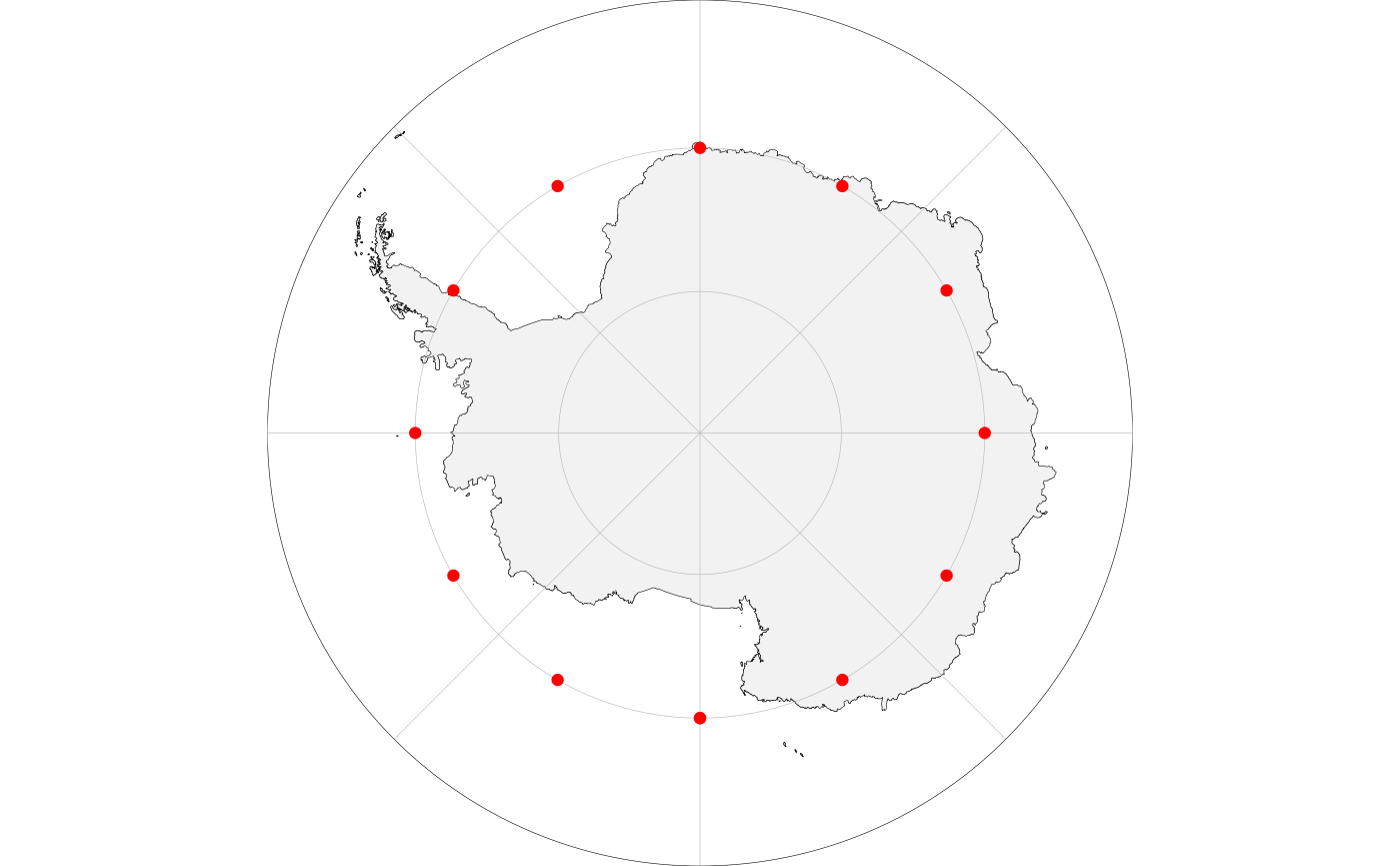

Graticules (the grid lines) can be removed by setting the grid.col to NA. Axis labels can be manipulated using standard ggplot code:

basemap(limits = c(124, 148, 31, 50), grid.col = NA) + 
  labs(x = NULL, y = "Only latitude for you, ...")

Add scale bar and north arrow

Scale bar and north arrows can be added using the ggspatial functions:

basemap(limits = c(-75, -45, 62, 78), rotate = TRUE) + 
  ggspatial::annotation_scale(location = "br") + 
  ggspatial::annotation_north_arrow(location = "tr", which_north = "true") 

Note that the north arrow in the example above points toward north where it is placed and that the direction of north varies as shown by the meridians. The scale bar is correct at 71 \(\circ\)N latitude as specified by the projection (crs = 3995) for Arctic stereographic maps.

Modifying basemap objects

The objects produced by the basemap function are standard ggplot objects with the difference that relevant information used in mapping is added to attributes of the object:

p <- basemap(-60)
names(attributes(p))

#> [1] "names"      "class"      "bathymetry" "glaciers"   "limits"    
#> [6] "polarmap"   "map.grid"   "crs"

Accessing the attributes allow custom modifications of maps produced by the basemap function. See the Reordering layers section as an example.

Reordering layers

Sometimes there is a need to move land, glacier, and grid layers on top of spatial data added on a basemap. This can be done using the reorder_layers function. This example uses Norwegian fishing regions (Hovedområder f.o.m. 2018), which can be downloaded from the Norwegian Directorate of Fisheries data portal (use “ESRI shapefile” option). The example works for any spatial polygons with crs information, however.

The Norwegian fishing regions are included as an example dataset in the ggOceanMaps package. You can add any data you want using the sf::st_read function.

data(fdir_areas)

basemap(fdir_main_areas) + 
  ggspatial::annotation_spatial(fdir_main_areas, fill = NA)

The initial plot draws the polygons. Note how the polygon boundaries are partly on land. We want to eventually hide them under land. We also add region labels and color the polygons based on their area to demonstrate the capabilities of sf, ggplot2, ggspatial and ggOceanMaps:

labels <- suppressWarnings(sf::st_centroid(fdir_main_areas))
fdir_main_areas$area <- as.numeric(sf::st_area(fdir_main_areas))/1e9 # calculate area in 1000 km2

p <- basemap(fdir_main_areas) +
  geom_sf(data = fdir_main_areas, aes(fill = area)) +
  geom_sf_text(data = labels, aes(label = main_area), size = FS(8), fontface = 2) +
  scale_fill_distiller(name = "Area\n(1000 km2)",
                       palette = "Spectral", na.value = "white",
                       limits = c(0, 500), oob = scales::squish)

reorder_layers(p)

Ideally, the region labels should not go under land. This can be fixed by plotting the labels on top of the reordered ggplot object. To demonstrate how to reorder layers, we do this manually here:

p <- reorder_layers(p)
tmp <- sapply(p$layers, function(k) !is.null(k$mapping$label)) # the layer with label mapping
p$layers <- c(p$layers[-which(tmp)], p$layers[which(tmp)])
p

Contolling the plotting order of graticules

Graticules are plotted using ggplot2::coord_sf() and are regarded as the panel element in the ggplot2::theme(). Note that also background color is included in the panel element (see the next section). The ggOceanMaps::theme_map() function, which is automatically executed together with every basemap() and qmap() command, controls the position of the graticules and they are set on top by default:

basemap(limits = c(-20, 15, 50, 70), grid.col = "red", grid.size = 1)

To move the graticules under all layers, use the panel.ontop argument in ggplot2::theme():

basemap(limits = c(-20, 15, 50, 70), grid.col = "red", grid.size = 1) + 
  theme(panel.ontop = FALSE)

Sometimes there is a need to control the position of graticules in between layers. At the time of writing, ggplot does not offer a straightforward way to do this, but we can use the code from ggplot2::coord_sf() to make the graticules:

p <- basemap(limits = c(-20, 15, 50, 70), grid.col = NA) + # without graticules 
  geom_sf(data = ices_areas, aes(fill = SubArea), show.legend = FALSE) 

# Make the graticules:
lims <- attributes(p)$limits 
graticule <- sf::st_graticule(
  c(lims[1], lims[3], lims[2], lims[4]), 
  crs = attributes(p)$crs,
  lon = seq(-180, 180, 15), lat = seq(-90, 90, 5))

# Plot
reorder_layers(p) +
  geom_sf(data = graticule, color = "grey70", size = LS(0.5)) + # graticules
  coord_sf(xlim = lims[1:2], ylim = lims[3:4], # redefine limits
           crs = attributes(p)$crs) +
  # labels on top of graticules
  geom_sf_label(
    data = suppressWarnings(sf::st_centroid(sf::st_make_valid(ices_areas))), 
    aes(label = Area_Full)
  )

An exception are the polar maps for which graticules are drawn by ggOceanMaps (because ggplot2 graticules for those maps were bugged some years ago when writing the function; this part requires a revision at some point).

X <- basemap_data(60)

basemap(60, grid.col = NA) +
  geom_sf(
    data = X$map.grid$lon.grid.lines, 
    color = "red", size = 1) +
  geom_sf(
    data = X$map.grid$lat.grid.lines, 
    color = "red", size = 1) +
  geom_sf(
    data = X$shapefiles$land, 
    fill = "grey60", color = "black", size = 0.1)

Coloring the ocean (background)

Similarly, the ggplot2::theme() panel element allows coloring the ocean:

basemap(expand.grid(lon = c(-129, -124), lat = c(49, 53)), grid.col = "red", grid.size = 0.5) + 
  theme(panel.background = element_rect(fill = "lightblue"),
        panel.ontop = FALSE) 

If you want the graticules on top, you’ll need to define them manually because, both, the background and the grid, are contained in the same ggplot element called panel:

p <- basemap(expand.grid(lon = c(-129, -124), lat = c(49, 53)), grid.col = NA) + 
  theme(panel.background = element_rect(fill = "lightblue"),
        panel.ontop = FALSE) 

# Make the graticules:
lims <- attributes(p)$limits 
graticule <- sf::st_graticule(
  c(lims[1], lims[3], lims[2], lims[4]), 
  crs = attributes(p)$crs,
  lon = attributes(p)$map.grid$lon.breaks, 
  lat = attributes(p)$map.grid$lat.breaks
)

# Plot
p + 
  geom_sf(data = graticule, color = "red", size = LS(1)) + # graticules
  coord_sf(xlim = lims[1:2], ylim = lims[3:4], # redefine limits
           crs = attributes(p)$crs) 

Add a fill scale on top of bathymetry

basemap(c(-20, 15, 50, 70), bathymetry = TRUE) + 
  annotation_spatial(ices_areas, aes(fill = Area_Full))
#> Error in `f()`:
# ! Insufficient values in manual scale. 75 needed but only 9 provided.
# Run `rlang::last_error()` to see where the error occurred.

This error comes because ggplot does not allow two color scales with similar mapping in one plot. The issue can be evaded by using contour bathymetry:

basemap(c(-20, 15, 50, 70), bathymetry = TRUE, 
        bathy.style = "contour_blues", legends = FALSE) + 
  annotation_spatial(ices_areas, aes(fill = Area_Full), alpha = 0.4) + 
  theme(legend.position = "none")

Or by using the ggnewscale package to make the data fill mapping disconnected from that in basemap:

basemap(limits = c(-20, 15, 50, 70), bathymetry = TRUE, 
        bathy.style = "poly_greys") +
  ggnewscale::new_scale_fill() +
  annotation_spatial(ices_areas, aes(fill = Area_Full), alpha = 0.4) + 
  theme(legend.position = "none")

Add longitude and latitude labels to a polar map

Since adding longitude and latitude labels to polar maps requires some manual fiddling for each map, there is no premade solution for this. Instead, you can do this using the sf package:

library(sf); library(dplyr)

p <- basemap(-60, shapefiles = "Antarctic")

p + 
  geom_text(
    data =
      attributes(p)$map.grid$lat.grid.lines %>% 
      sf::st_coordinates() %>% 
      as.data.frame() %>% 
      dplyr::filter(X == -180) %>%
      dplyr::add_row(X = -180, Y = -90, L1 = 3, L2 = 1) %>% 
      transform_coord(proj.out = attributes(p)$crs, bind = TRUE),
    aes(x = lon.proj, y = lat.proj, label = paste0(abs(Y), "\u00B0S"))
  ) +
  geom_text(
    data =
      attributes(p)$map.grid$lon.grid.lines %>% 
      sf::st_coordinates() %>% 
      as.data.frame() %>% 
      dplyr::filter(Y == -60) %>%
      dplyr::mutate(Y = -63) %>% 
      transform_coord(proj.out = attributes(p)$crs, bind = TRUE),
    aes(x = lon.proj, y = lat.proj, 
        label = ifelse(sign(X) == 1, paste0(abs(X), "\u00B0E"), 
                       paste0(abs(X), "\u00B0W"))
    )
  ) +
  theme(plot.margin = margin(0.25, 0.25, 0.25, 0.25, "cm"))

Custom shapefiles

The ggOceanMaps package uses vector (spatial polygon) data for land and glaciers to make the plotting more efficient and to produce sharp images at any resolution. Further, both vector and raster bathymetries can be used. Each of these layers have to be defined using the same projection. Since the shapefiles are large and generating them may require long processing time, it is most convenient to save them in a Rdata file in sf format and load them to the memory when used to make a map. Useful sources for spatial data are:

Vector data

• Natural Earth Data provides polygon data in relatively high detail for the entire Earth. Used as data-source for land and glacier shapes throughout the package, except for the most detailed maps.
• European Environment Agency provides high-resolution land shapes for Europe.
• Norwegian Mapping Authority provides high-resolution spatial data for mainland Norway and Svalbard.
• Norwegian Polar Institute provides high-resolution vector data for Norwegian polar regions.

Raster data for bathymetry

• GEBCO Compilation Group (2019) GEBCO 2019 15-arcsecond grid. The highest resolution open bathymetry grid available at the moment. Referred to as “GEBCO data”.
• ETOPO1 15 Arc-Second Global Relief Model. Can also be accessed using the marmap::getNOAA.bathy (see Section 1). Referred to as “NOAA data” and “ETOPO data”.

There are probably more sources which the author has not needed yet. Please send an email to add more options to the list. The bathymetry datasets are large and require vectorization before they can be plotted in ggplot2 within a reasonable time.

Here we go through how to plot customized shapefiles for the Barents Sea as an example. A similar procedure can be applied to any region in the world.

Bathymetries

The Natural Earth Data provides bathymetry vector data, which can be readily used in ggOceanMaps. The contours in that dataset are, however, not very practical for marine biology and fisheries in shallow seas such as the Barents Sea. Download the ETOPO dataset as Ice surface elevation NetCDF to a folder in your computer. It may be beneficial to make a “GIS” or “Shapefiles” folder where you store similar datasets for later use. Whether you use ice or bed-rock surface does not matter for this example as there are no glaciers under the sea-level within the region of interest. In any case, this choice has no visual effect because land and glaciers will be plotted on top of the bathymetry, but the ice surface option will lead to smaller file size.

The bathymetry needs first to be reclassified and formatted for the consequent vectorization step. First, we need to define the location of the ETOPO dataset and to find limits for our region in decimal degrees. The limits can be found using the basemap function. It is advised to use slightly wider limits than the region of interest.

etopoPath <- "" # Replace by the path to the folder where the ETOPO1 grd file is located.
lims <- c(-8, 65, 68, 82)
projection <- "EPSG:32636"
basemap(limits = lims)

We also need to define an appropriate projection. We will use the UTM 36N zone projection, which is approximately in the middle of our area of interest. We define higher resolution contour in depths 0-500 m because our area of interest is relatively shallow. The raster_bathymetry function is relatively slow for large data. The aggregation.factor argument can be used to reduce file size but will influence the resolution of the resulting shapefile (higher factors lead to a lower resolution).

rb <- raster_bathymetry(bathy = paste(etopoPath, "ETOPO1_Ice_g_gmt4.grd", sep = "/"),
                        depths = c(50, 100, 200, 300, 500, 1000, 1500, 2000, 4000, 6000, 10000), 
                        proj.out = projection, 
                        boundary = lims
)

Now we have the bathyRaster object which can be vectorized:

class(rb)
names(rb)
raster::plot(rb$raster)

The vectorization is done using the vector_bathymetry function. The drop.crumbs and remove.holes parameters can be used to reduce the file size, while the smooth parameter makes the contours look smoother under high zoom levels. Note that the smoothing of raster cell edges is completely arbitrary and may lead to map contours that do not exist in reality.

bs_bathy <- vector_bathymetry(rb)
sp::plot(bs_bathy)

Land shapes

Land shapes could theoretically be defined from the bathymetry raster (depth = 0). Nevertheless, since the 10m Natural Earth Data vectors are of high resolution, there has been no need to write a function to do this. We use Natural Earth Data instead. Download the Natural Earth Data Land and Minor Islands vectors to your “GIS” or “Shapefiles” folder and define folder paths under:

NEDPath <- "" # Natural Earth Data location
outPath <- "" # Data output location

Once done, we go ahead and process the shapefiles:

world <- rgdal::readOGR(paste(NEDPath, "ne_10m_land/ne_10m_land.shp", sep = "/"))
islands <- rgdal::readOGR(paste(NEDPath, "ne_10m_minor_islands/ne_10m_minor_islands.shp", sep = "/"))
world <- rbind(world, islands)

bs_land <- clip_shapefile(world, lims)
bs_land <- sp::spTransform(bs_land, CRSobj = sp::CRS(projection))
rgeos::gIsValid(bs_land) # Has to return TRUE, if not use rgeos::gBuffer
bs_land <- rgeos::gBuffer(bs_land, byid = TRUE, width = 0)
sp::plot(bs_land)

Glacier shapes

Download the Natural Earth Data Glaciated Areas vectors to your NEDPath.

glaciers <- rgdal::readOGR(paste(NEDPath, "ne_10m_glaciated_areas/ne_10m_glaciated_areas.shp", sep = "/"))
rgeos::gIsValid(glaciers) # Needs buffering
glaciers <- rgeos::gBuffer(glaciers, byid = TRUE, width = 0)

bs_glacier <- clip_shapefile(glaciers, lims)
bs_glacier <- sp::spTransform(bs_glacier, CRSobj = sp::CRS(projection))
rgeos::gIsValid(bs_glacier)
sp::plot(bs_glacier)

Plotting the shapefiles using basemap

Now that we have the shapefiles, we can save them to a file so that we do not run the script above every time we plot a map using custom shapefiles.

save(bs_bathy, bs_land, bs_glacier, file = paste(outPath, "bs_shapes.rda", sep = "/"), compress = "xz")

The shapefiles can now be plotted using the basemap function:

basemap(shapefiles = list(land = bs_land, glacier = bs_glacier, bathy = bs_bathy), bathy.style = "poly_blues", glaciers = TRUE)

The list elements land, glacier and bathy are required, but glacier and bathy can be set to NULL if bathymetry and glaciers are set to FALSE, respectively. This means that you are not forced to define bathymetries and glaciers for your custom shapefile maps if plotting them is not desired. Note how the map becomes plotted outside its actual limits. This issue will hopefully be fixed in the future. The map can be limited using the limits or data arguments as any basemap:

basemap(limits = c(10, 53, 70, 80), shapefiles = list(land = bs_land, glacier = bs_glacier, bathy = bs_bathy), bathy.style = "poly_blues", glaciers = TRUE)

Known issues

The land and glacier shapes do not get dissolved correctly when projecting from decimal degrees:

basemap(60, glaciers = TRUE)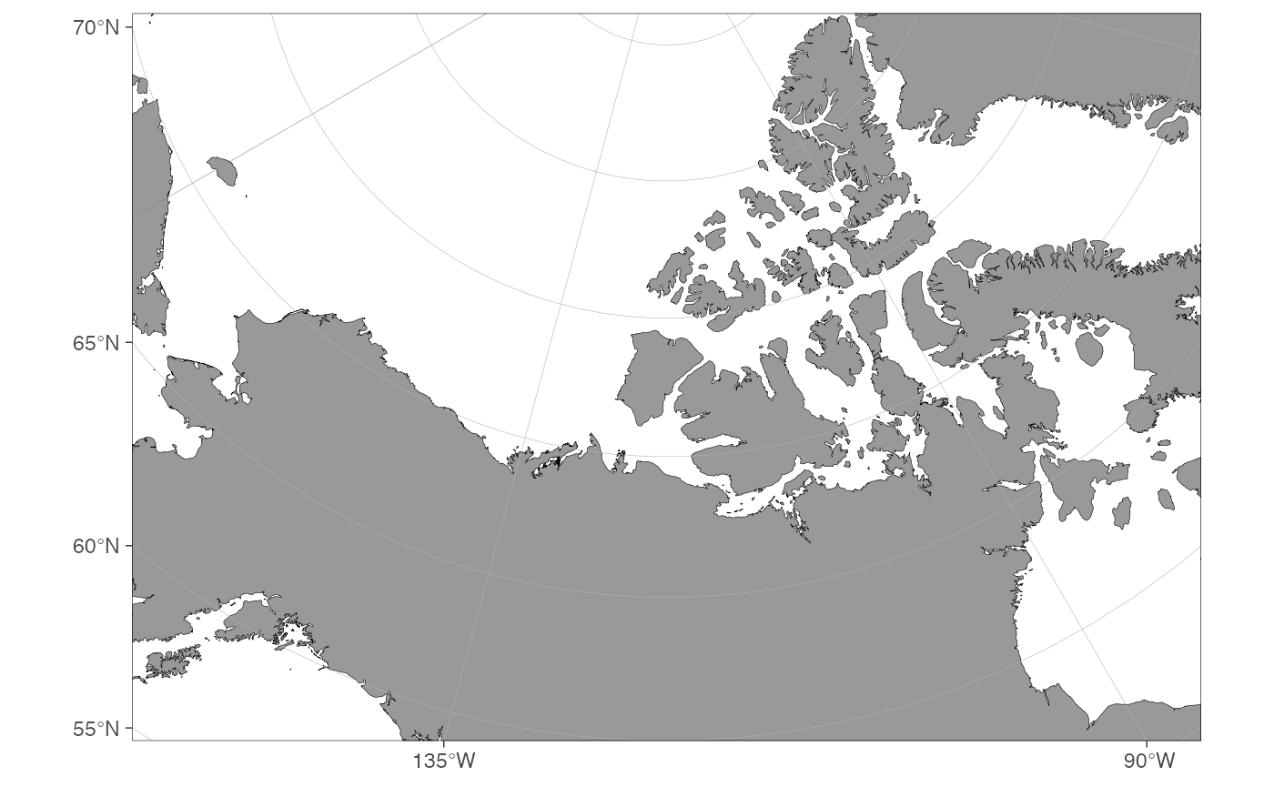

A solution until the issue has been fixed is to use projected downloadable shape files:

basemap(60, glaciers = TRUE, shapefiles = "Arctic")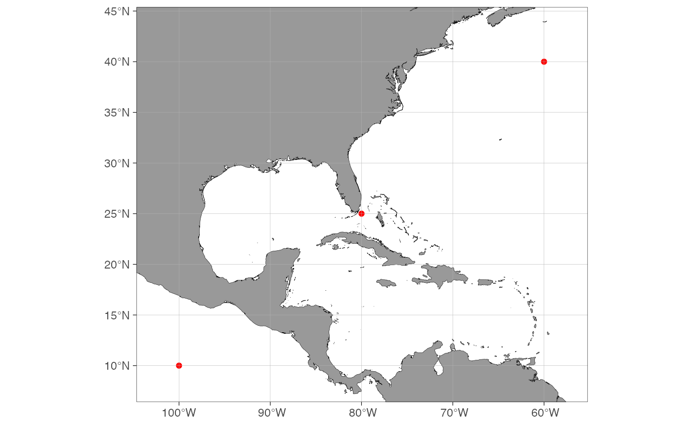

Citations and data sources

The data used by the package are not the property of the Institute of Marine Research nor the author of the package. It is, therefore, important that you cite the data sources used in a map you generate with the package. Please see here for a list of data sources.

Please cite the package whenever maps generated by the package are published. For up-to-date citation information, please use:

citation("ggOceanMaps")

#> To cite package 'ggOceanMaps' in publications use:
#> 
#>   Vihtakari M (2024). _ggOceanMaps: Plot Data on Oceanographic Maps
#>   using 'ggplot2'_. R package version 2.2.0,
#>   <https://mikkovihtakari.github.io/ggOceanMaps/>.
#> 
#> A BibTeX entry for LaTeX users is
#> 
#>   @Manual{,
#>     title = {ggOceanMaps: Plot Data on Oceanographic Maps using 'ggplot2'},
#>     author = {Mikko Vihtakari},
#>     year = {2024},
#>     note = {R package version 2.2.0},
#>     url = {https://mikkovihtakari.github.io/ggOceanMaps/},
#>   }