Customising shapefiles

Mikko Vihtakari (Institute of Marine Research)

22 June, 2026

library(ggOceanMaps)

When the premade maps do not cover your region at the resolution you need, you can supply your own land, glacier, and bathymetry layers to basemap(). This article covers four ways to build them: clipping an existing layer, deriving land and bathymetry from a raster, reading Norwegian Geonorge depth data, and vectorising a WCS bathymetry fetch to pair with a premade land set. The figures below are pre-rendered (see dev/make_customising_shapefiles_vignette_figs.R) so this article builds without downloading data or re-running heavy spatial operations.

For where the bathymetry data come from (shipped, ggOceanMapsLargeData, your own raster, or live WCS), see the Bathymetry article. This one is about turning data you already have into ggOceanMaps shapefiles.

The shapefiles argument

basemap() accepts a named list of three sf/stars objects:

basemap(
  limits = c(-5, 10, 50, 60),
  shapefiles = list(land = my_land, glacier = NULL, bathy = my_bathy),
  bathymetry = TRUE
)

• land — an sf polygon layer (required).
• glacier — an sf polygon layer, or NULL if you have none.
• bathy — either a stars raster (continuous/binned raster styles) or an sf polygon layer of depth contours (vector styles), or NULL.

All three must share one projection. basemap() uses that CRS for the map, so there is no need to call coord_sf() yourself. shapefile_list() shows the same structure for the built-in sets and is a good template.

Clipping an existing layer

clip_shapefile() crops any sf polygon layer to a bounding box. It is the quickest way to make a regional land layer from a larger one (e.g. the shipped dd_land):

land <- clip_shapefile(
  dd_land,
  limits = c(-5, 10, 50, 60) # c(xmin, xmax, ymin, ymax), decimal degrees
)

basemap(shapefiles = list(land = land, glacier = NULL, bathy = NULL))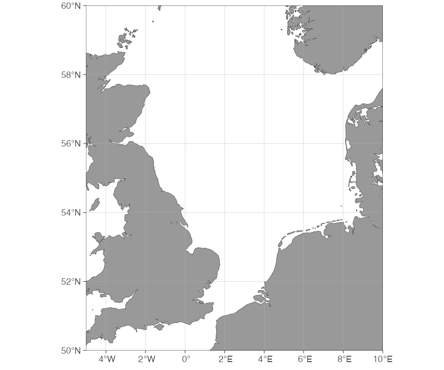

Figure: Land layer clipped to the North Sea.

limits are interpreted with proj.limits (decimal degrees by default). For a projected input layer, pass the limits in that projection’s units and set proj.limits to its CRS, or keep limits in degrees and let the function reproject the clip box. Use return.boundary = TRUE to get the clipping polygon back for inspection.

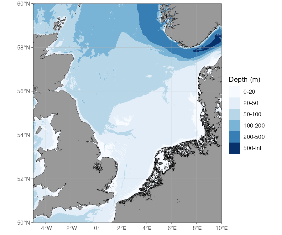
Building land + bathymetry from a raster

A single source grid (GEBCO, ETOPO, IBCAO, …) gives you a matched land and bathymetry pair. The pipeline is raster_bathymetry() first, then vector_bathymetry() and/or vector_land(). This example reuses the North Sea region from the clipping example above, with depth breaks suited to its mostly-shallow shelf and the deeper Norwegian Trench along the Norwegian coast:

# 1. Read + crop + sign-flip the grid; bin to depth contours.
rb <- raster_bathymetry(
  bathy = "path/to/your/bathymetry.nc",
  depths = c(20, 50, 100, 200, 500), # contour break points
  boundary = c(-5, 10, 50, 60), # crop early to save memory
  estimate.land = TRUE # keep land cells for vector_land()
)

raster_bathymetry() returns a bathyRaster: a list with the processed raster (a stars object) and the depth intervals. Feed that object to the vectorisers:

# 2a. Depth-contour polygons for the vector bathymetry styles
vb <- vector_bathymetry(rb, drop.crumbs = NULL)

# 2b. Land polygons extracted from the same grid
vl <- vector_land(rb, drop.crumbs = NULL)

# 2c. Normalise the CRS to plain EPSG:4326 (see note below).
vb <- sf::st_transform(vb, 4326)
vl <- sf::st_transform(vl, 4326)

# vector_bathymetry() also polygonizes the "land" class added by
# estimate.land -- drop it, it belongs in vl.
vb <- vb[vb$depth != "land", ]
vb$depth <- droplevels(vb$depth)

# 3. Plug both into basemap(). Vector bathymetry needs an explicit
# bathy.style ("pb" here); bathymetry = TRUE alone assumes a raster.
basemap(
  limits = c(-5, 10, 50, 60),
  shapefiles = list(land = vl, glacier = NULL, bathy = vb),
  bathy.style = "pb"
)

Figure: Land and bathymetry vectorised from a GEBCO raster, North Sea.

Normalise the CRS (step 2c). GEBCO, ETOPO and IBCAO NetCDF grids are read with a non-standard “unknown” geographic CRS — an unnamed datum with latitude/longitude (rather than longitude/latitude) axis order. basemap() clips and renders the map in the land layer’s CRS, and that axis-swapped CRS makes the rectangular clip box slant slightly, leaving a thin uncovered wedge along the southern map edge. Transforming vb and vl to plain EPSG:4326 before plotting removes it. Do this on the vectorised layers, not via proj.out in raster_bathymetry(): reprojecting the raster there turns it into a curvilinear grid that vector_bathymetry() cannot polygonise.

vector_land() takes the same bathyRaster as vector_bathymetry() and the same cleanup arguments (drop.crumbs, remove.holes, smooth). Leave drop.crumbs at NULL when you need vl and vb to share a coastline: the two functions apply it independently, so a shared non-NULL threshold can drop a small island from one layer without dropping the matching sliver of shallow water from the other, leaving tiny gaps at the coast. drop.crumbs is still useful to shrink file size when you don’t need the two layers to line up exactly — it is in km², so scale it down for small regions; a city-block-scale area needs something like 0.01, not 10. To keep continuous (unbinned) raster bathymetry instead of depth-contour polygons, pass depths = NULL to raster_bathymetry() and use rb$raster directly as bathy (skipping vector_bathymetry()).

Save the processed layers so you do not re-run the heavy raster step every session:

save(vb, vl, file = "north_sea_shapes.rda")
# later:
load("north_sea_shapes.rda")

Reading Geonorge depth data

For Norwegian waters, the Geonorge depth-area vector shapefiles can be downloaded as .gml and include a matching land layer in the same file, so both sit at the same resolution and CRS. geonorge_bathymetry() reads the depth layer; sf::st_read() with layer = "Landareal" reads the land:

gb <- geonorge_bathymetry("path/to/Dybdedata.gml")
land <- sf::st_read("path/to/Dybdedata.gml", layer = "Landareal")

# Use the data's own extent and projection.
bb <- sf::st_bbox(gb)
limits <- c(bb["xmin"], bb["xmax"], bb["ymin"], bb["ymax"])

basemap(
  limits = limits,
  shapefiles = list(land = land, glacier = NULL, bathy = gb),
  bathy.style = "pb"
)

Figure: Geonorge depth data for Oslo municipality.

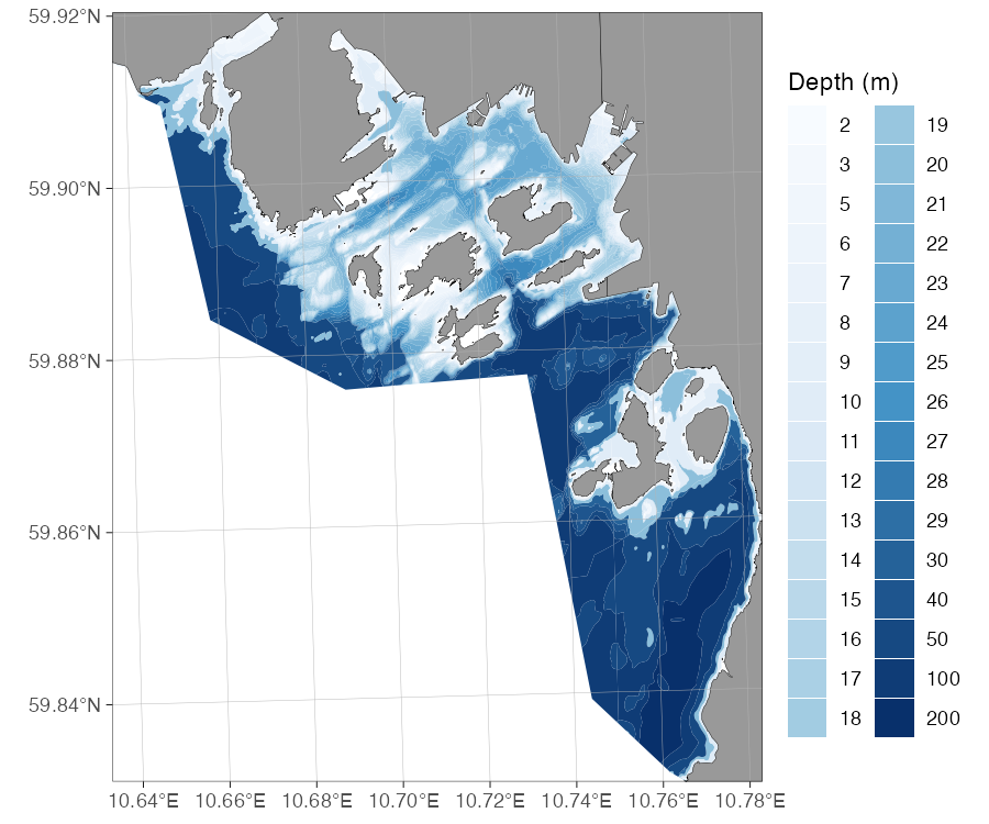
This example uses Oslo municipality’s depth-area tile, a small dataset showing the harbour, Bygdøy, and the surrounding islands. By default geonorge_bathymetry() reads the "dybdeareal" layer; pass layer = if your file uses a different name, and verbose = TRUE to see the reading steps.

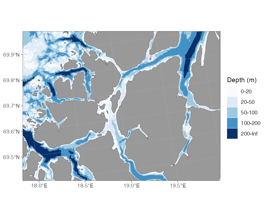
Pairing a WCS fetch with a premade shapefile set

wcs_bathymetry() fetches bathymetry on demand from a Web Coverage Service and returns a continuous bathyRaster, but it always discards land (it calls raster_bathymetry(ras, depths = NULL) internally). Since this section is about making new shapefiles rather than just plotting a raster, the example below vectorises the fetched bathymetry into depth-contour polygons — the same cut() + vector_bathymetry() pattern as the raster section above — and pairs it with the premade "Europe" land set, which is a better match for EMODnet’s ~115 m resolution than the shipped dd_land:

tromso <- c(18, 20, 69.4, 69.9) # area to display
fetch <- c(17.5, 20.5, 69.3, 70) # slightly wider fetch box (see note below)
bathy <- wcs_bathymetry(fetch, source = "emodnet")

# wcs_bathymetry() always returns depths = NULL (continuous), so bin it
# into depth-contour classes by hand before vectorising.
breaks <- c(-Inf, 20, 50, 100, 200, Inf)
labels <- c("0-20", "20-50", "50-100", "100-200", "200-Inf")
rb <- list(raster = cut(bathy$raster, breaks, labels = labels))
class(rb) <- "bathyRaster"
vb <- vector_bathymetry(rb, drop.crumbs = NULL)

# Reproject the bathymetry to the "Europe" land set's CRS (EPSG:3035) and clip
# the land to the bathymetry extent, so both are in the plotted projection.
europe_land <- load_map_data(shapefile_list("Europe"))$land
vb <- sf::st_transform(vb, sf::st_crs(europe_land))
land <- sf::st_crop(sf::st_make_valid(europe_land), sf::st_bbox(vb))

basemap(
  limits = tromso,
  shapefiles = list(land = land, glacier = NULL, bathy = vb),
  bathy.style = "pb"
)

Figure: Bathymetry fetched live from EMODnet around Tromsø, vectorised and paired with the premade Europe land set.

Fetch a little wider than you display. The map is plotted in the "Europe" land set’s CRS (EPSG:3035), but a WCS request is a decimal-degree (EPSG:4326) box. Its straight lat/lon edges slant once reprojected to 3035, so a fetch box exactly equal to the map limits leaves uncovered slivers in the projected map’s corners. Requesting a slightly larger fetch box than the tromso area you display covers the whole panel. Clipping the land to st_bbox(vb) keeps it in the same projection as the bathymetry and the map, so the clipping happens in the plotted CRS rather than across a reprojection.

load_map_data() is the internal helper basemap() itself uses to load and, if needed, download a premade set’s layers — calling it directly here gets just the "Europe" land polygons without its default bathymetry. For a quick look at a raw WCS fetch without vectorising, pair bathy$raster directly with dd_land and use bathymetry = TRUE instead, as in wcs_bathymetry()’s own examples.

See also

• Bathymetry — choosing and obtaining the underlying data.
• Premade shapefiles — how the built-in sets were built, as a fuller worked example.
• Cookbook — compact copy-pasteable versions of these recipes.