Premade maps
Mikko Vihtakari (Institute of Marine Research)
22 June, 2026
Source:vignettes/premade-maps.Rmd
premade-maps.RmdOverview
ggOceanMaps plots maps from pre-made shapefiles.
Most of the time you do not need to think about them:
basemap() picks the right set automatically from the
limits (or data) you give it. This article
shows the maps that ship with — or are downloadable for — the package,
and the projection each uses.
The available sets are listed by shapefile_list():
shapes <- shapefile_list("all")
datapath <- path.expand(getOption("ggOceanMaps.datapath"))
userpath <- path.expand(getOption("ggOceanMaps.userpath", ""))
shapes[] <- lapply(shapes, function(x) {
  if (!is.character(x)) return(x)
  x <- gsub(datapath, "<ggOceanMaps.datapath>", x, fixed = TRUE)
  if (nzchar(userpath)) {
    x <- gsub(userpath, "<ggOceanMaps.userpath>", x, fixed = TRUE)
  }
  x
})
shapes
#>                     name                                  land
#> 1    ArcticStereographic    <ggOceanMaps.datapath>/arctic_land
#> 2 AntarcticStereographic <ggOceanMaps.datapath>/antarctic_land
#> 3          DecimalDegree                               dd_land
#> 4               Svalbard  <ggOceanMaps.datapath>/svalbard_land
#> 5                 Europe    <ggOceanMaps.datapath>/europe_land
#>                                    glacier
#> 1    <ggOceanMaps.datapath>/arctic_glacier
#> 2 <ggOceanMaps.datapath>/antarctic_glacier
#> 3        <ggOceanMaps.datapath>/dd_glacier
#> 4  <ggOceanMaps.datapath>/svalbard_glacier
#> 5                                     <NA>
#>                                                                                    bathy
#> 1    dd_rbathy|<ggOceanMaps.datapath>/dd_rbathy_cont|<ggOceanMaps.datapath>/arctic_bathy
#> 2 dd_rbathy|<ggOceanMaps.datapath>/dd_rbathy_cont|<ggOceanMaps.datapath>/antarctic_bathy
#> 3        dd_rbathy|<ggOceanMaps.datapath>/dd_rbathy_cont|<ggOceanMaps.datapath>/dd_bathy
#> 4  dd_rbathy|<ggOceanMaps.datapath>/dd_rbathy_cont|<ggOceanMaps.datapath>/svalbard_bathy
#> 5        dd_rbathy|<ggOceanMaps.datapath>/dd_rbathy_cont|<ggOceanMaps.datapath>/dd_bathy
#>     crs                                      limits
#> 1  3995                                       c(30)
#> 2  3031                                      c(-35)
#> 3  4326                       c(-180, 180, -90, 90)
#> 4 32633 c(402204.7, 845943.9, 8253526.1, 8978517.5)
#> 5  3035        c(943609, 7601958, -375446, 6825119)
#>                                                                      path
#> 1 https://github.com/MikkoVihtakari/ggOceanMapsLargeData/raw/master/data/
#> 2 https://github.com/MikkoVihtakari/ggOceanMapsLargeData/raw/master/data/
#> 3 https://github.com/MikkoVihtakari/ggOceanMapsLargeData/raw/master/data/
#> 4 https://github.com/MikkoVihtakari/ggOceanMapsLargeData/raw/master/data/
#> 5 https://github.com/MikkoVihtakari/ggOceanMapsLargeData/raw/master/data/
Each row is a named shapefile set with a coordinate reference system
(crs), a default extent (limits), and the
names of its land / glacier / bathymetry objects. You can force a
particular set with the first argument or the shapefiles
argument (partial matching works, so "Arctic" resolves to
"ArcticStereographic"):
basemap(shapefiles = "Svalbard", bathymetry = TRUE)Low-resolution global data (dd_land,
dd_rbathy) ship with the package. The higher-resolution
regional sets live in the ggOceanMapsLargeData
repository and are downloaded automatically on first
use to getOption("ggOceanMaps.datapath"). Set that
option to a permanent folder in your .Rprofile so the files
are reused across sessions; otherwise they land in
tempdir() and are re-downloaded each session.
Standard maps (selected automatically)
These three sets cover the whole globe and are chosen automatically
from the latitude range of your limits: polar-stereographic
projections near the poles, decimal degrees elsewhere. See the user manual for the exact selection
rule.
Decimal degree
The default map uses decimal degrees (EPSG:4326) and Natural Earth 1:10m land and minor-island polygons.
basemap("DecimalDegree", bathymetry = TRUE, glaciers = TRUE)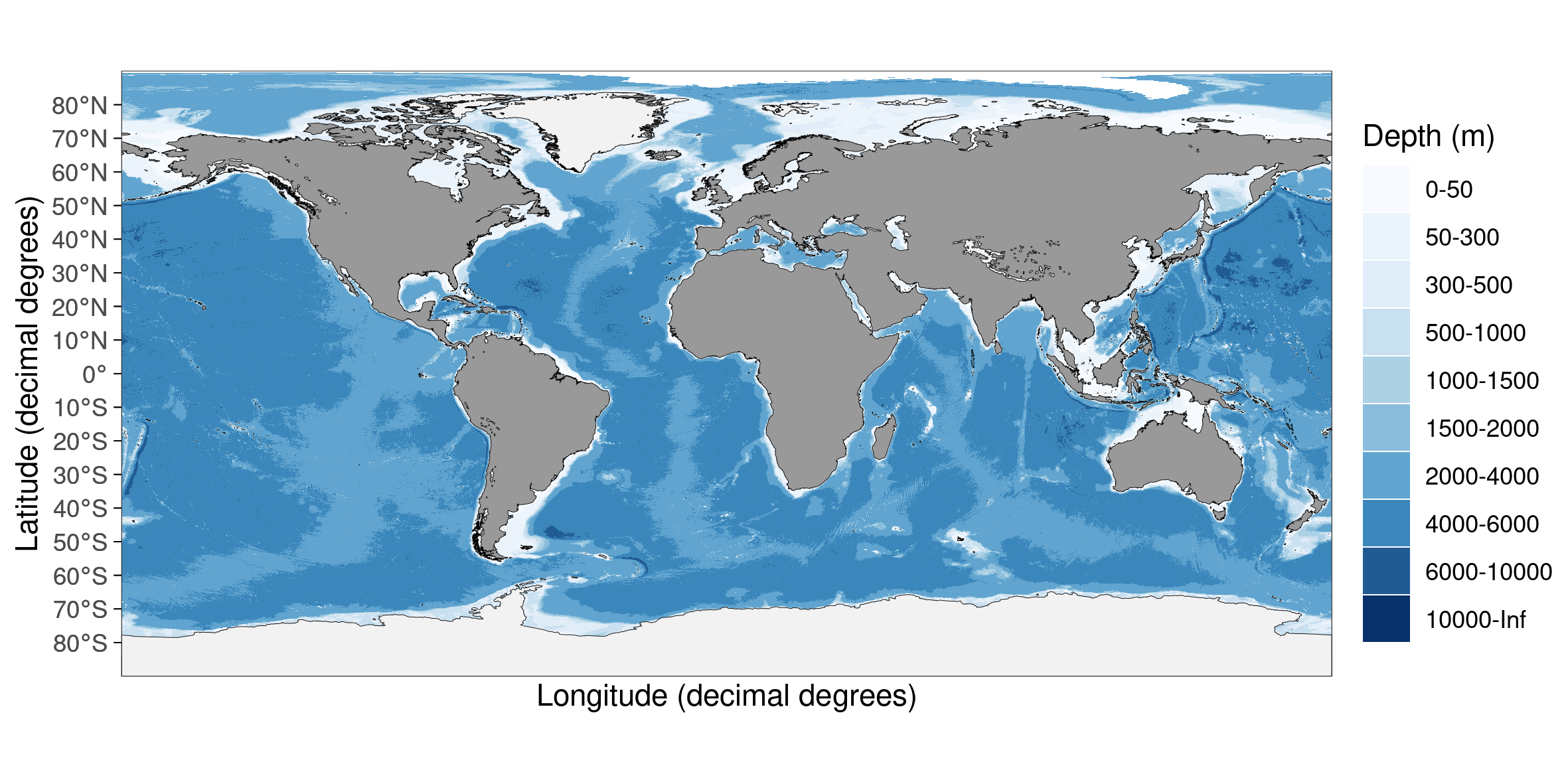
Arctic Stereographic
Used automatically when the map sits in the high north (EPSG:3995). Land and glacier polygons and vector bathymetry are downloaded from ggOceanMapsLargeData on first use.
basemap("ArcticStereographic", bathymetry = TRUE, glaciers = TRUE)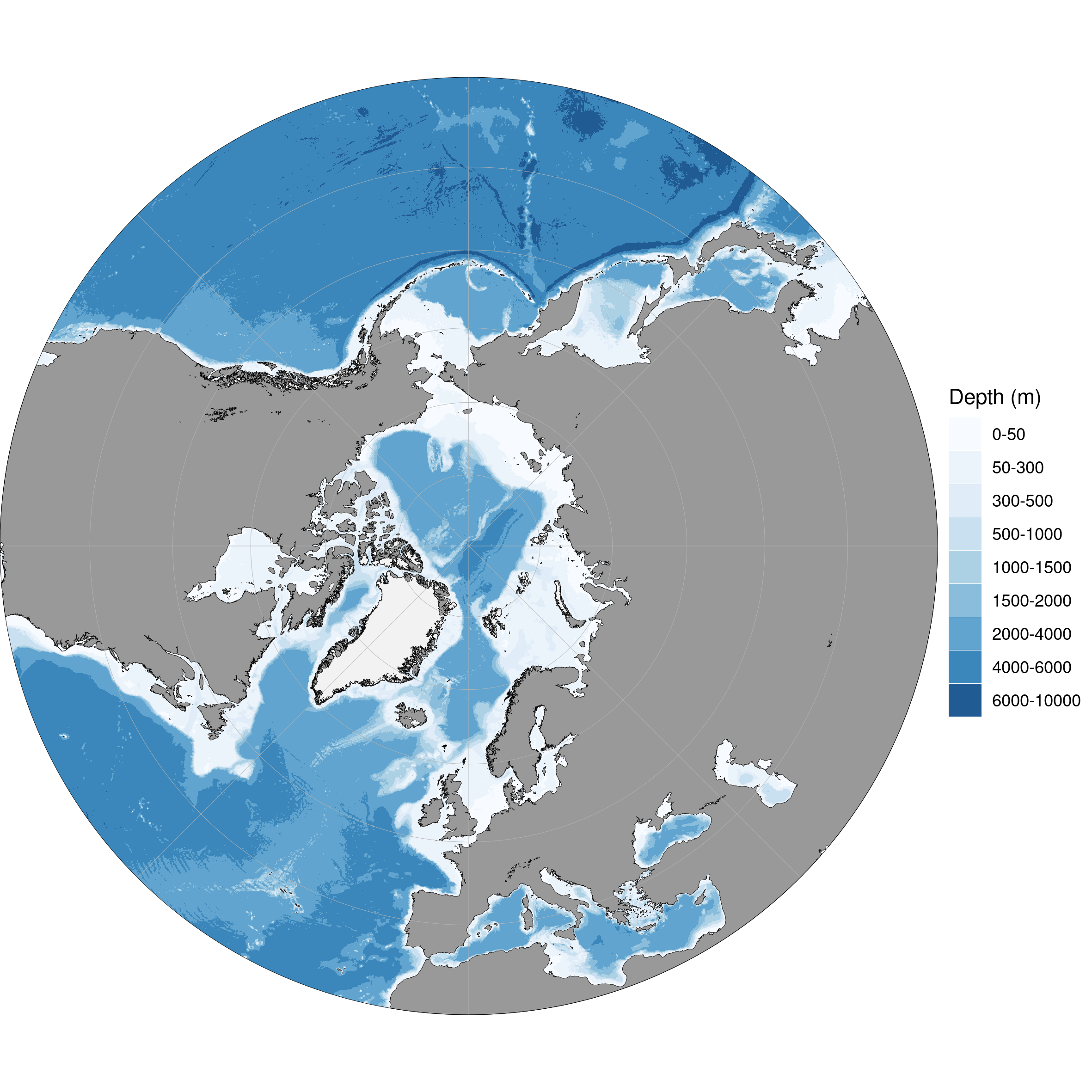
Antarctic Stereographic
The southern equivalent (EPSG:3031).
basemap("AntarcticStereographic", bathymetry = TRUE, glaciers = TRUE)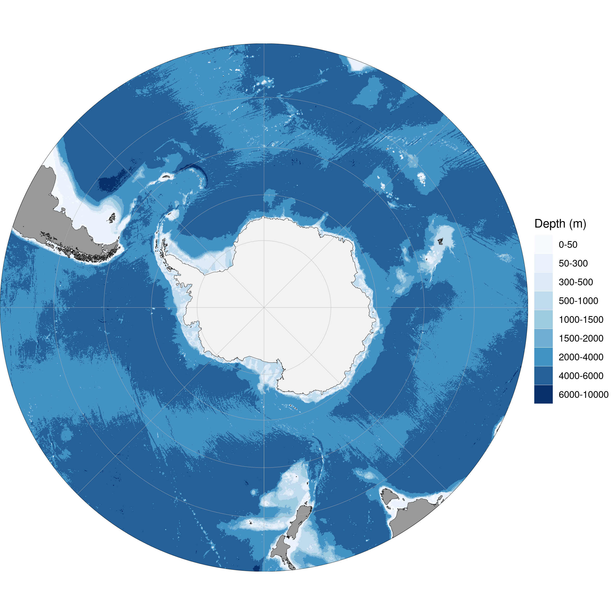
Detailed regional maps
Higher-resolution sets for regions the package author works in. They are downloaded from ggOceanMapsLargeData when first requested. The detailed shapefiles can be large: find your limits with the standard maps first, and export to a file rather than plotting into the screen device for big extents.
Only a handful of regions have a dedicated high-resolution set. If
your area of interest is not in the list above — or you need finer land
or bathymetry than the standard maps provide — you can build your own
land and bathymetry shapefiles and pass them to basemap()
via the shapefiles argument. See the Customising shapefiles article
for the full workflow.
Europe
A detailed European coastline (EPSG:3035) based on the EEA coastline. Useful for coastal maps around the European seas. Can be paired with EMODnet bathymetry for ~115 m resolution bathymetric maps (see New features in v3 for example).
basemap(shapefiles = "Europe")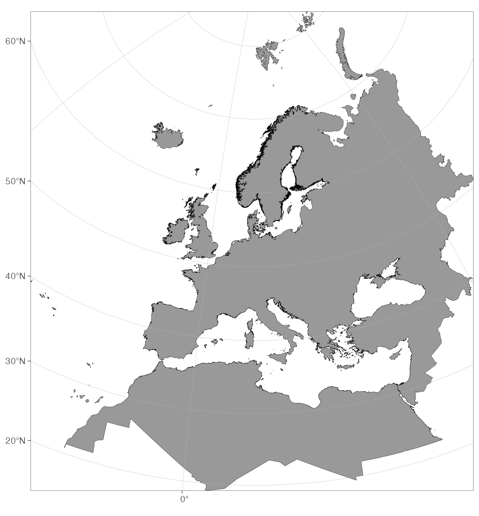
The Europe land polygons are downloaded from ggOceanMapsLargeData on first use.
Svalbard
A detailed Svalbard map (EPSG:32633), originally from the PlotSvalbard package. The function asks to download the data the first time you use it.
basemap("Svalbard", glaciers = TRUE)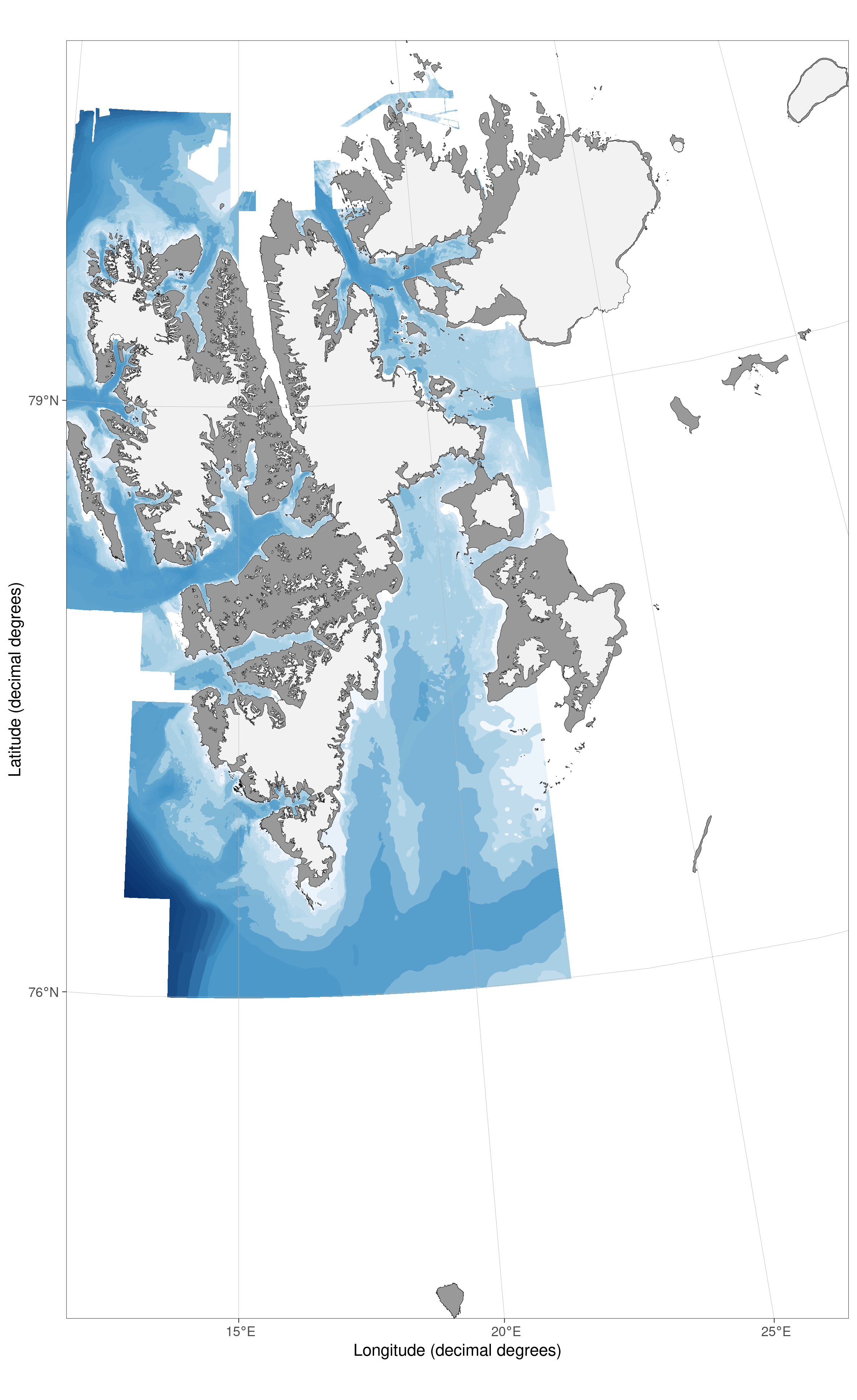
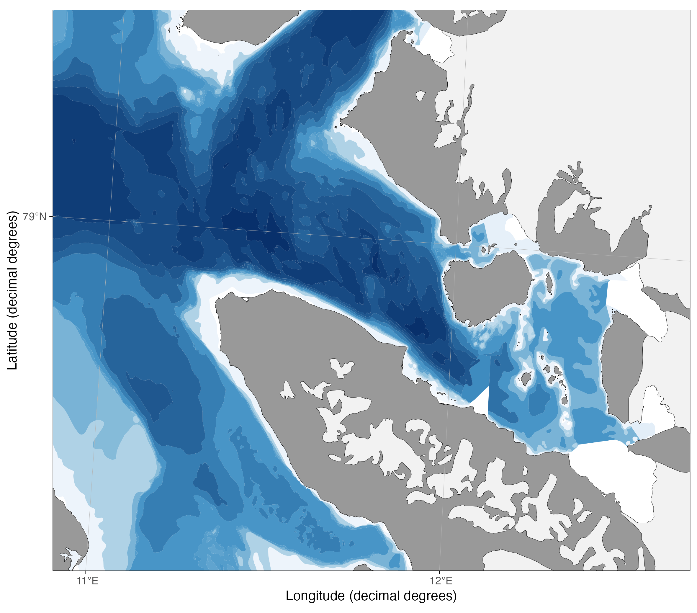
Zooming to Kongsfjorden. Svalbard and Europe maps can be paired with the EMODnet bathymetry:
basemap(
  limits = c(10.9, 12.65, 78.83, 79.12),
  bathy.style = "wemb",
  shapefiles = "Svalbard",
  legends = FALSE,
  glaciers = TRUE
)
Citing the data
The data used by the package are not the property of the Institute of Marine Research nor the package author. Please cite the data sources used in any map you generate. See the data-source list for the references.