Adding graphical elements

Mikko Vihtakari (Institute of Marine Research)

22 June, 2026

library(ggOceanMaps)
library(ggplot2)

basemap() returns a standard ggplot2 object, so points, paths, polygons, labels, and custom scales are added with +. The one thing to watch is the coordinate system: at high latitudes, and whenever crs is set, the map axes are projected metres rather than longitude and latitude. Add geographic coordinates to those maps through transform_coord(), ggspatial::geom_spatial_*(), or geom_sf(), which reproject on the fly.

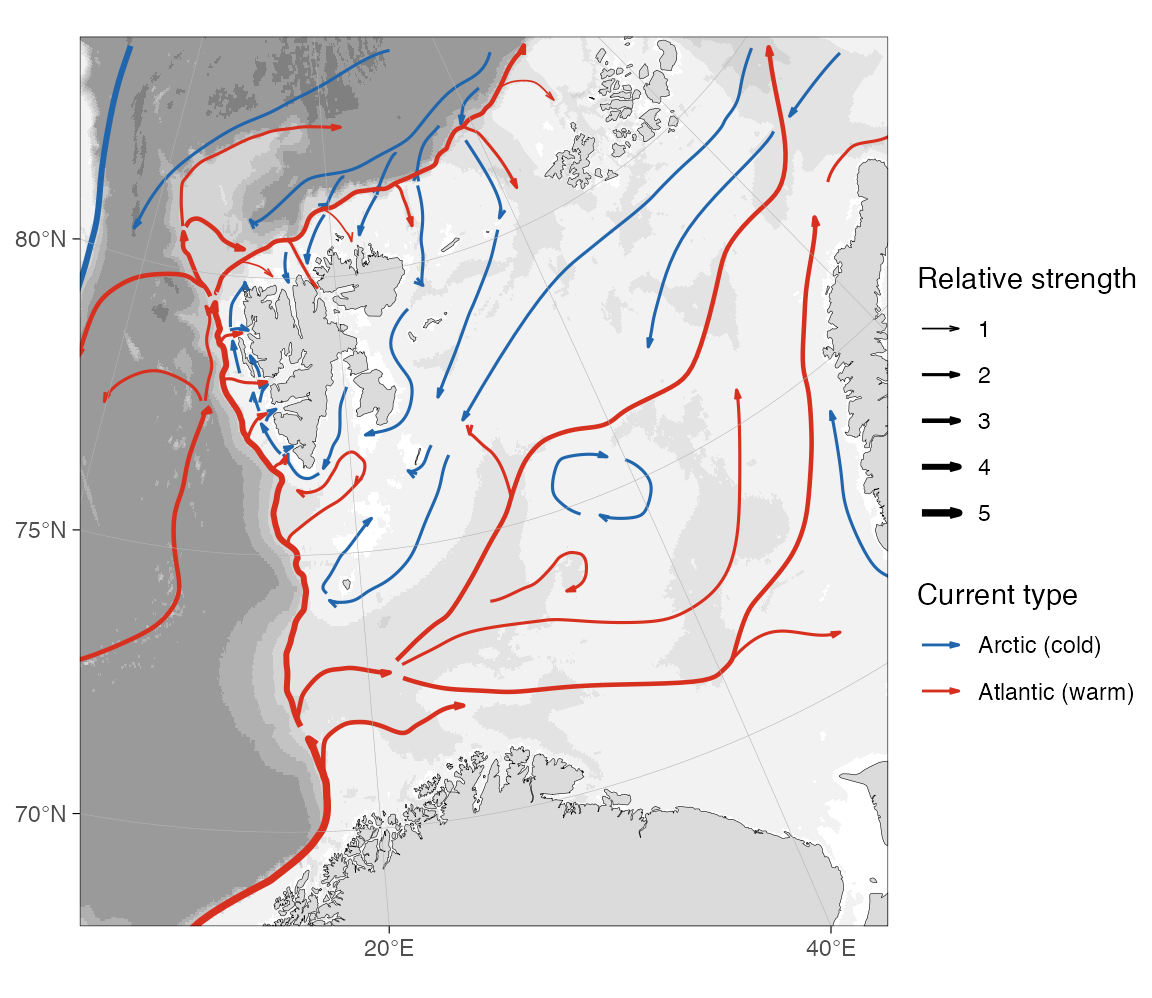
Schematic current arrows

The Barents-Sea-currents repository provides publication-style “Figure 1” current arrows for the Barents Sea and North Atlantic. The example below downloads the tidy Barents Sea CSV, builds one line per arrow, smooths it, and draws it with geom_path(). Smoothing happens in projected metres rather than in longitude/latitude, which would exaggerate the curves near the pole.

barents_url <- paste0(
  "https://raw.githubusercontent.com/MikkoVihtakari/",
  "Barents-Sea-currents/master/tabular/barents_currents.csv"
)
barents_file <- file.path(tempdir(), "barents_currents.csv")

if (!file.exists(barents_file)) {
  try(
    download.file(barents_url, barents_file, quiet = TRUE, mode = "wb"),
    silent = TRUE
  )
}

# Offline fallback bundled with the vignette.
if (!file.exists(barents_file)) {
  barents_file <- file.path("data", "barents_currents.csv")
}

cur <- read.csv(barents_file)
head(cur)
#>   id      long      lat order        group size     type
#> 1  0  5.306694 66.34752     1 Atlantic_0.1    5 Atlantic
#> 2  0  5.306694 66.34752     2 Atlantic_0.1    5 Atlantic
#> 3  0  6.448918 66.73568     3 Atlantic_0.1    5 Atlantic
#> 4  0  9.080173 67.53121     4 Atlantic_0.1    5 Atlantic
#> 5  0 10.656624 68.29049     5 Atlantic_0.1    5 Atlantic
#> 6  0 13.568487 69.01010     6 Atlantic_0.1    5 Atlantic

Each arrow is a group of ordered nodes. Assemble them into one LINESTRING per arrow, reproject to the map CRS, and smooth the nodes into curves with smoothr::smooth().

library(sf)

cur <- cur[order(cur$group, cur$order), ]
parts <- split(cur, cur$group)

arrows <- st_sf(
  do.call(rbind, lapply(parts, function(d) d[1, c("group", "type", "size")])),
  geometry = st_sfc(
    lapply(parts, function(d) st_linestring(as.matrix(d[, c("long", "lat")]))),
    crs = 4326
  )
)
arrows <- smoothr::smooth(st_transform(arrows, 32633), method = "spline")

# Tidy projected coordinates for geom_path().
co <- as.data.frame(st_coordinates(arrows))
cur_lines <- data.frame(
  x = co$X,
  y = co$Y,
  group = arrows$group[co$L1],
  type = arrows$type[co$L1],
  size = arrows$size[co$L1]
)

The arrows sit on top of the basemap, so they would otherwise be drawn over land. reorder_layers() pushes the land, glacier, and grid layers back on top, tucking the arrows under the coastline.

current_arrow <- arrow(
  type = "open",
  angle = 15,
  ends = "last",
  length = unit(0.25, "lines")
)

reorder_layers(
  basemap(
    limits = c(5, 45, 68, 83.5),
    crs = 32633,
    bathy.style = "rbg",
    land.col = "grey86",
    legends = c(FALSE, TRUE)
  ) +
    geom_path(
      data = cur_lines,
      aes(x, y, group = group, colour = type, linewidth = size),
      arrow = current_arrow
    ) +
    scale_colour_manual(
      "Current type",
      values = c(Atlantic = "#d7301f", Arctic = "#2166ac"),
      labels = c(Atlantic = "Atlantic (warm)", Arctic = "Arctic (cold)")
    ) +
    scale_linewidth("Relative strength", range = c(0.3, 1.3))
)

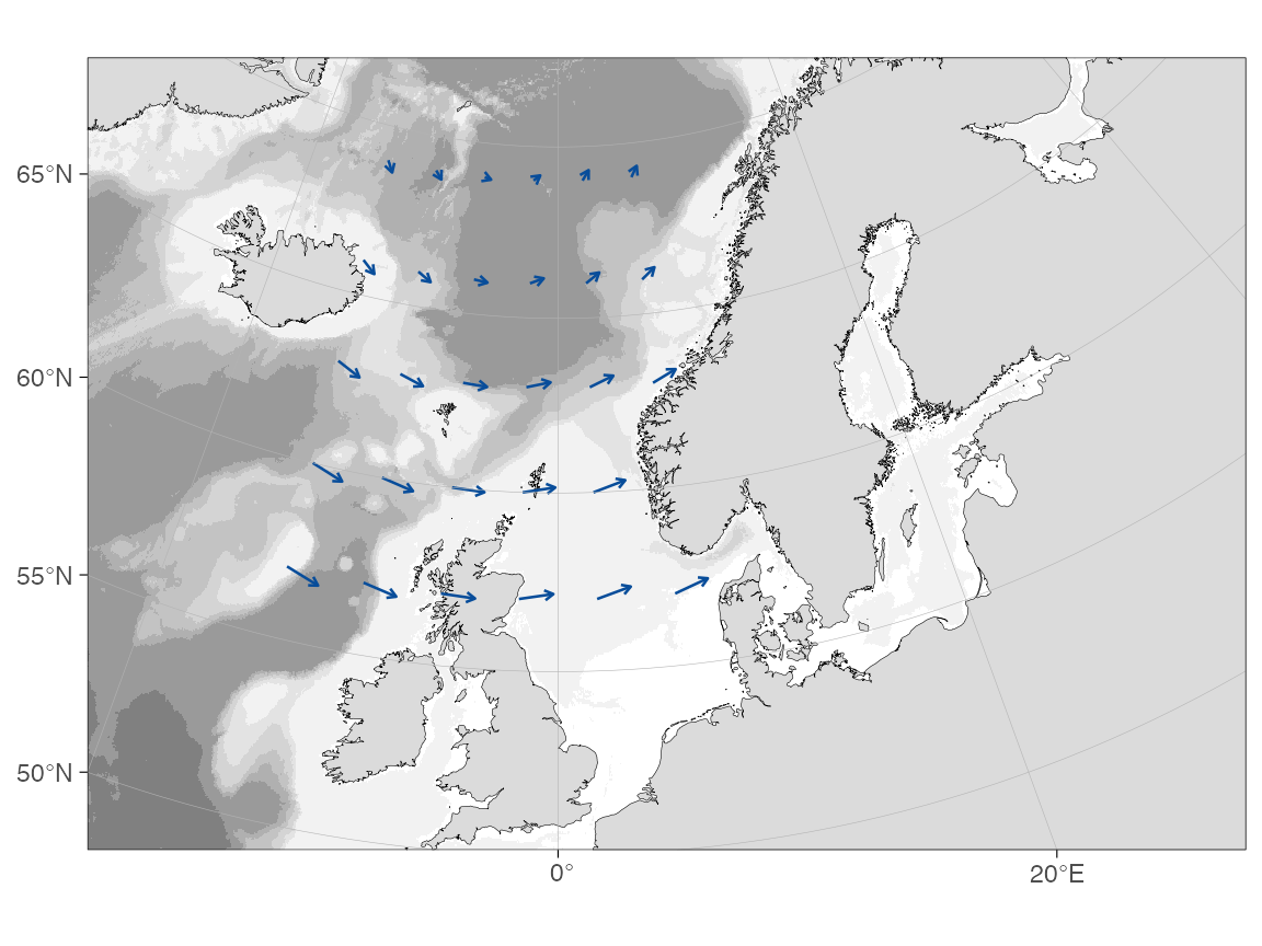
Velocity fields

For a gridded velocity field, compute the arrow endpoints, transform both the start and end points to the basemap CRS, and draw the result with geom_segment(). The example uses a small synthetic field filtered to ocean positions; the same pattern applies after reading u and v from a NetCDF file.

grd <- expand.grid(lon = seq(-14, 6, by = 4), lat = seq(57, 69, by = 3))
grd <- dist2land(grd, binary = TRUE, dist.col = "ocean", verbose = FALSE)
grd <- grd[grd$ocean, ]

grd$u <- 0.35 + 0.25 * cos((grd$lat - 58) / 4) # eastward component
grd$v <- 0.20 * sin((grd$lon + 5) / 6) # northward component

# Display scale only: a 1 m/s vector is drawn as 50 hours of drift.
km_per_ms <- 50 * 3.6
grd$lon_end <- grd$lon +
  (grd$u * km_per_ms) / (111.32 * cos(grd$lat * pi / 180))
grd$lat_end <- grd$lat + (grd$v * km_per_ms) / 110.57

# Transform both ends to the basemap projection.
start <- transform_coord(
  grd,
  lon = "lon",
  lat = "lat",
  proj.out = 3995,
  bind = TRUE
)
end <- transform_coord(
  grd,
  lon = "lon_end",
  lat = "lat_end",
  proj.out = 3995,
  new.names = c("lon_end.proj", "lat_end.proj")
)
grd <- cbind(start, end)

basemap(
  limits = c(-20, 30, 50, 70),
  bathy.style = "rbg",
  land.col = "grey86",
  legends = FALSE
) +
  geom_segment(
    data = grd,
    aes(x = lon.proj, y = lat.proj, xend = lon_end.proj, yend = lat_end.proj),
    arrow = arrow(length = unit(0.12, "cm"), type = "open"),
    colour = "#084d9a",
    linewidth = 0.45
  )

On a decimal-degree map the same code works without the transform_coord() calls. Use those maps only when the basemap itself is in EPSG:4326; many high-latitude limits select a polar projection automatically.

Pie charts

Pie charts can be drawn as ordinary polygons. This avoids an extra plotting dependency and keeps the coordinate units explicit: after projection the pie radius is in metres. The helper below turns a row of category counts into one polygon per slice.

pie_polygons <- function(data, cols, x, y, r, n = 60) {
  out <- vector("list", nrow(data) * length(cols))
  k <- 1

  for (i in seq_len(nrow(data))) {
    values <- as.numeric(data[i, cols])
    values[is.na(values)] <- 0
    prop <- values / sum(values)
    starts <- c(0, cumsum(prop)[-length(prop)]) * 2 * pi
    ends <- cumsum(prop) * 2 * pi

    for (j in seq_along(cols)) {
      theta <- seq(
        starts[j],
        ends[j],
        length.out = max(2, ceiling(n * prop[j]))
      )
      out[[k]] <- data.frame(
        id = data$id[i],
        slice = cols[j],
        x = c(
          data[[x]][i],
          data[[x]][i] + cos(theta) * data[[r]][i],
          data[[x]][i]
        ),
        y = c(
          data[[y]][i],
          data[[y]][i] + sin(theta) * data[[r]][i],
          data[[y]][i]
        ),
        part = paste(data$id[i], cols[j], sep = "_")
      )
      k <- k + 1
    }
  }

  do.call(rbind, out)
}

pies <- data.frame(
  id = c("A", "B", "C", "D"),
  lon = c(-8, 0, 4, 9),
  lat = c(56.5, 60, 63.5, 67.5),
  cod = c(45, 20, 60, 25),
  haddock = c(30, 50, 15, 35),
  saithe = c(25, 30, 25, 40)
)
slices <- c("cod", "haddock", "saithe")

pies <- transform_coord(pies, proj.out = 3995, bind = TRUE)
pies$r <- 90000 # metres
pie_df <- pie_polygons(pies, slices, x = "lon.proj", y = "lat.proj", r = "r")

basemap(
  limits = c(-12, 16, 54, 70),
  bathy.style = "rbg",
  land.col = "grey86",
  legends = FALSE
) +
  ggnewscale::new_scale_fill() +
  geom_polygon(
    data = pie_df,
    aes(x = x, y = y, group = part, fill = slice),
    colour = "white",
    linewidth = 0.15,
    alpha = 0.95
  ) +
  scale_fill_brewer("Species", palette = "Set2")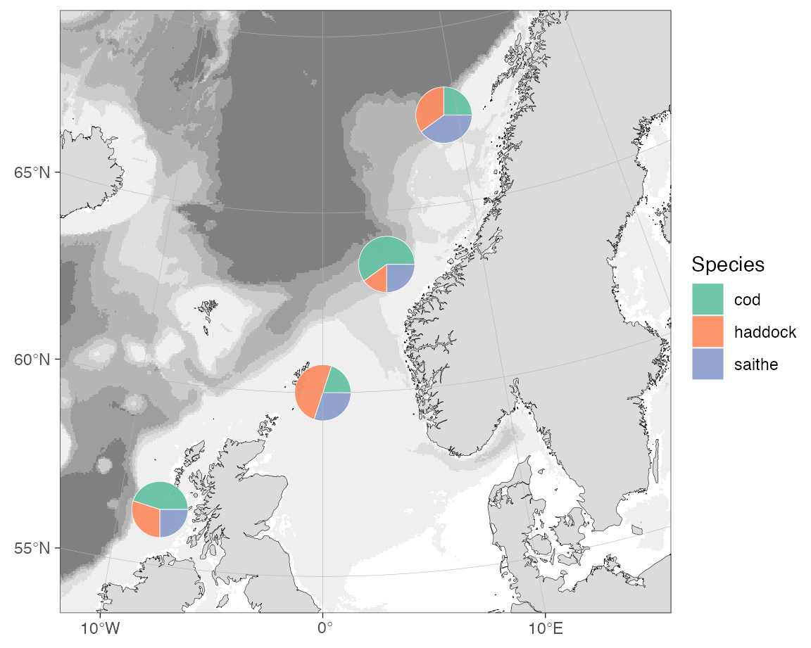

The basemap already maps bathymetry to fill, so insert ggnewscale::new_scale_fill() between the basemap and the pie layer to give the slices an independent fill scale.

Recolouring bathymetry

basemap() maps the binned bathymetry styles to a discrete fill scale and the continuous styles (rcb, rcg) to a continuous one. Either is recoloured by adding a matching ggplot2 fill scale after the basemap, exactly as in the Appearance section of the User manual.

basemap(c(11, 16, 67.3, 68.6), grid.col = NA, bathymetry = TRUE) +
  scale_fill_viridis_d("Depth (m)")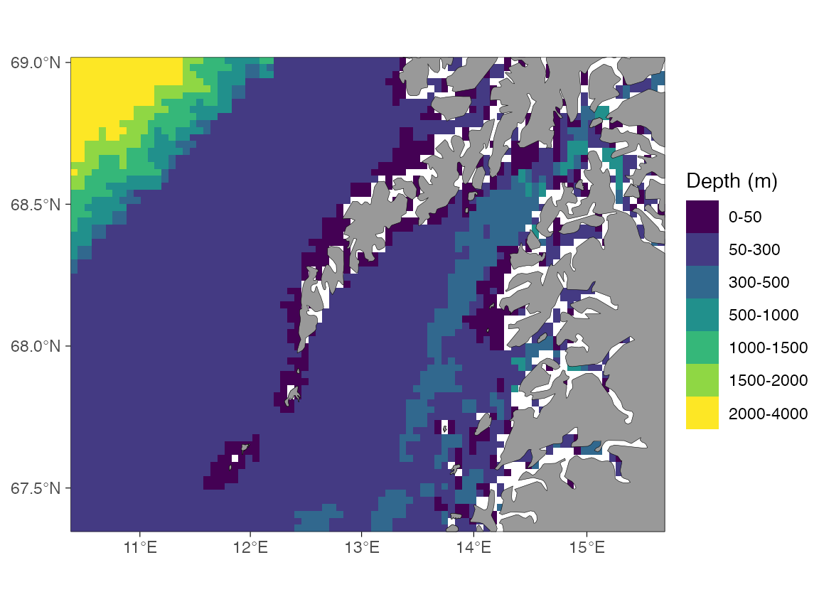

For a continuous style, use a continuous fill scale instead. scale_fill_stepsn() additionally lets you set your own breaks and a non-linear transformation, binning the continuous raster at plotting time without changing the data. (This example needs the higher-resolution continuous raster from ggOceanMapsLargeData; it is skipped when that file is not available.)

basemap(
  c(11, 16, 67.3, 68.6),
  grid.col = NA,
  bathy.style = "rcb",
  downsample = 5
) +
  scale_fill_stepsn(
    name = "Depth (m)",
    breaks = c(0, 50, 100, 200, 500, 1000),
    limits = c(0, NA),
    trans = "sqrt",
    colours = colorRampPalette(
      c("#F7FBFF", "#DEEBF7", "#9ECAE1", "#4292C6", "#08306B")
    )(5),
    na.value = "white"
  )

Custom depth bins with raster_bathymetry()

The scales above recolour bathymetry that ggOceanMaps has already prepared. To bin a raw depth raster into classes of your own, re-bin it with raster_bathymetry(): pass the cut points to depths and hand the returned binned raster straight to basemap() through shapefiles. Any grid that stars::read_stars() can open works — the example reads a local GEBCO file (see the Your own raster section of the Bathymetry article), cropped to the shelf off Lofoten.

# Your local GEBCO/ETOPO/IBCAO grid, e.g. set once with
# options(ggOceanMaps.userpath = "path/to/GEBCO_2025.nc")
gebco <- getOption("ggOceanMaps.userpath")

rb <- raster_bathymetry(
  gebco,
  depths = c(50, 100, 250, 500, 1000, 2000), # depth class boundaries
  boundary = c(11, 16, 67.3, 68.6), # crop to the map region
  estimate.land = TRUE, # keep land cells so vector_land() can use them
  verbose = FALSE
)

# Each depths value becomes a class boundary.
levels(rb$raster[[1]])

The standard grey land comes from a coarser global coastline, which can sit slightly off a high-resolution grid like GEBCO. Pull the land from the same raster with vector_land() so the coastline matches the bathymetry exactly — estimate.land = TRUE above kept the land cells for this. Drop that "land" class from the raster itself so it is not drawn as a depth bin. The binned raster then behaves like any binned bathymetry: switch it on with bathymetry = TRUE and recolour it with a discrete fill scale (a sequential ColorBrewer palette here).

# Land from the same grid lines up with the bathymetry.
land <- vector_land(rb)
land <- sf::st_transform(land, 4326) # normalise GEBCO's "unknown" CRS

# Drop the land class so the raster shows depth bins only.
v <- rb$raster[[1]]
v[as.character(v) == "land"] <- NA
rb$raster[[1]] <- droplevels(v)

basemap(
  limits = c(11, 16, 67.3, 68.6),
  shapefiles = list(land = land, glacier = NULL, bathy = rb),
  bathymetry = TRUE,
  grid.col = NA
) +
  scale_fill_brewer("Depth (m)", palette = "YlGnBu", na.value = "white")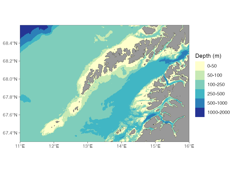

Figure: Custom depth bins off Lofoten, binned with raster_bathymetry() and coloured with a ColorBrewer YlGnBu palette.

raster_bathymetry() reports the intervals in rb$depth.invervals. The same binned raster can be turned into depth-contour polygons with vector_bathymetry() for the pre-made-shapefile workflow described in the Customising shapefiles article.