PlotSvalbard - User Manual
Mikko Vihtakari (Institute of Marine Research)
29 April, 2020
Source:vignettes/PlotSvalbard.Rmd
PlotSvalbard.Rmdlibrary(PlotSvalbard)
Plot research data from Svalbard on maps. R package version 0.9.2.
PlotSvalbard package provides functions to plot research data from Svalbard on high resolution maps in R. The package is based on ggplot2 and the functions can be expanded using ggplot syntax. The package contains also maps from other places in the Arctic, including polar stereographic maps of the Arctic.
Basemap
The basemap function is the generic plotting command in PlotSvalbard, and is analogous to empty ggplot() call. The basemap() call plots a map that is specified by the type argument. Data containing geographic information can be plotted on these maps using the ggplot2 layers separated by the + operator.
Map types
Map types are specified by the type argument in basemap() function. The list below shows all currently implemented map types.
Barents Sea
basemap("barentssea")
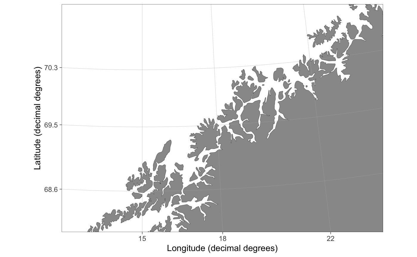
Barents Sea map also prints mainland Norway, but the projection is not optimal, and the resolution is quite low.
Limiting (zooming) the maps
Any basemap can be limited (or zoomed in) using the limits argument. The limits argument has to be either a numeric vector of length 4 or a character vector of length 3. Numeric vectors are used to constrain (zoom in) the maps using coordinates. Character vectors are used to automatically zoom into a dataset.
Manual limits
Achieved using a numeric vector. The first element defines the minimum longitude, the second element the maximum longitude, the third element the minimum latitude and the fourth element the maximum latitude of the bounding box. The coordinates have to be given as decimal degrees for Svalbard and Barents Sea maps and as UTM coordinates for pan-Arctic maps (see ?transform_coord).
Note that some map types are already limited, so if you are looking for a map of Kongsfjorden, using basemap("kongsfjorden") might be just what you need.
Automatic limits
Requires a character vector: the first element gives the object name of the data frame containing data to which the map should be limited, the second argument gives the column name of longitude data and the third argument the column name of latitude data. The map will be limited using rounded minimum and maximum floor and ceiling values for longitude and latitude and (hopefully) sensible rounding resolution depending on the size of the map. The limits.lon and limits.lat arguments can be used to override the default rounding.
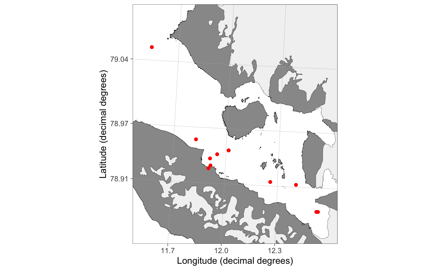
basemap(type = "svalbard", limits = c("kongsfjord_moorings", "Lon", "Lat")) +
  geom_point(data = kongsfjord_moorings, aes(x = lon.utm, y = lat.utm), color = "red")
Bathymetry
All basemaps support bathymetry, but the resolution of bathymetry shapefiles is varying. Bathymetry can be plotted using the bathymetry argument.
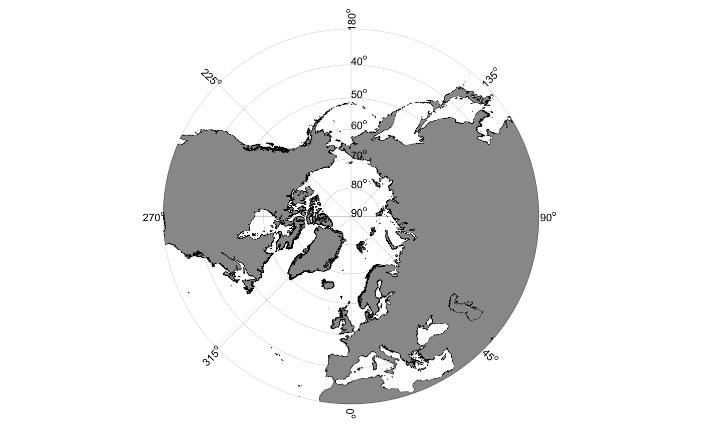
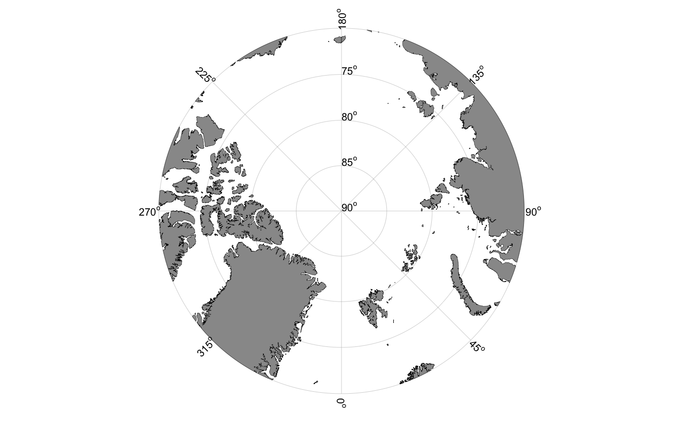
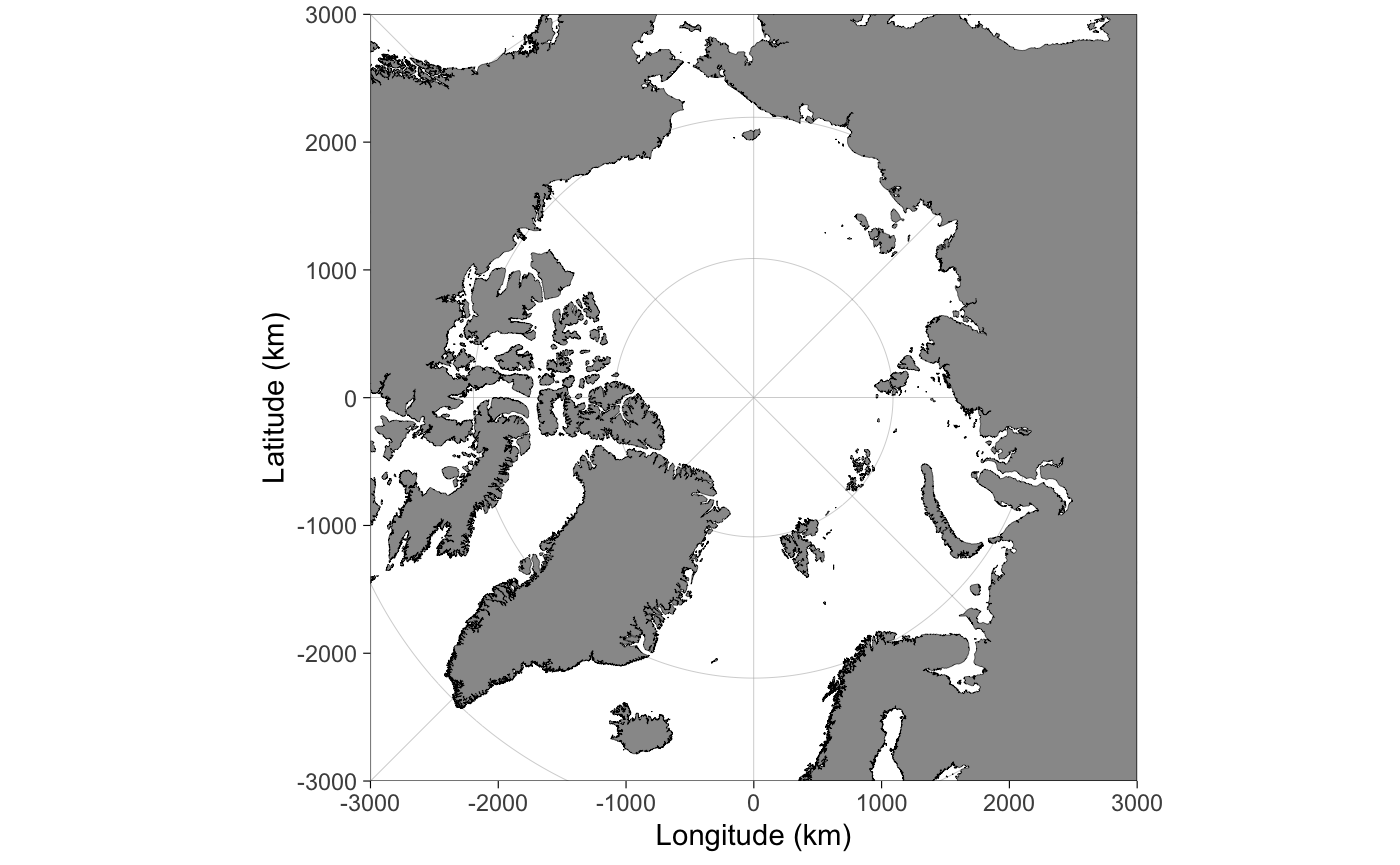
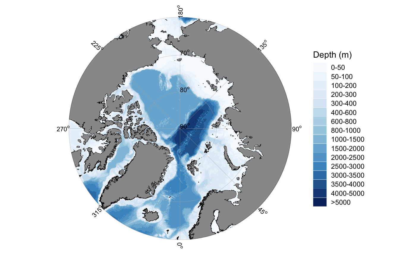
basemap("panarctic", limits = 60, bathymetry = TRUE)
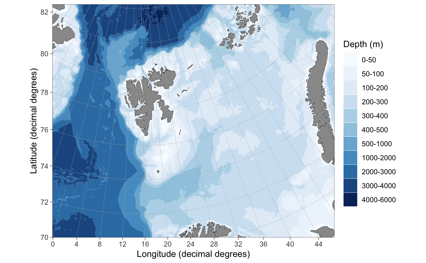
basemap("barentssea", bathymetry = TRUE)
Detailed bathymetry shapes
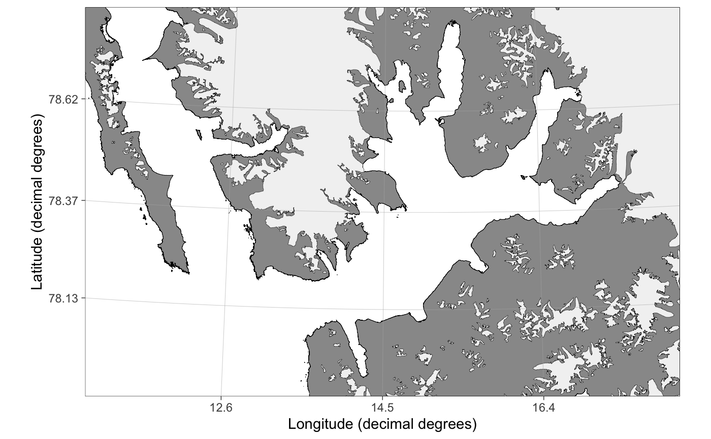
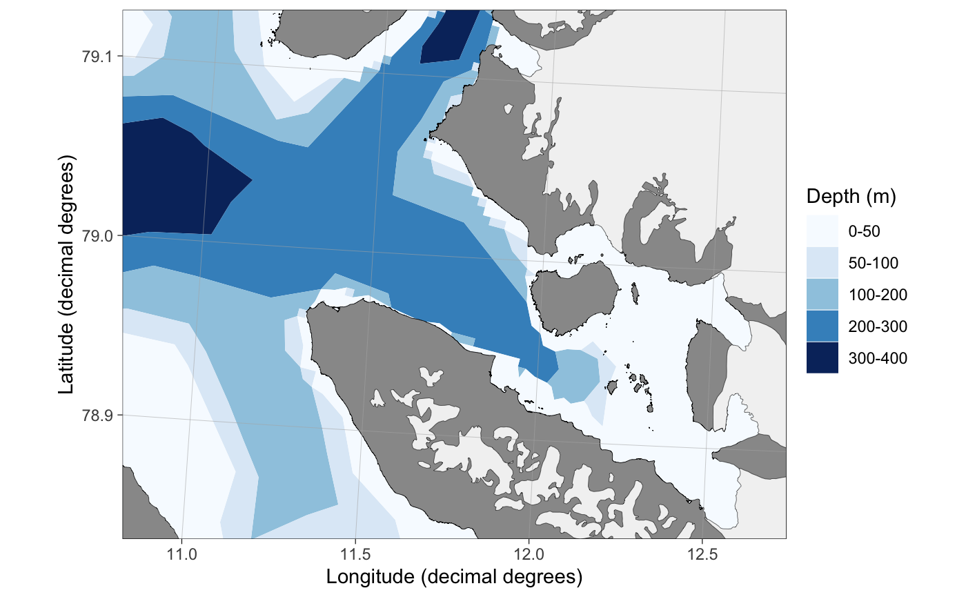
The default bathymetry shapefile is too low resolution to be used inside Svalbard fjords:
basemap("kongsfjorden", bathymetry = TRUE)
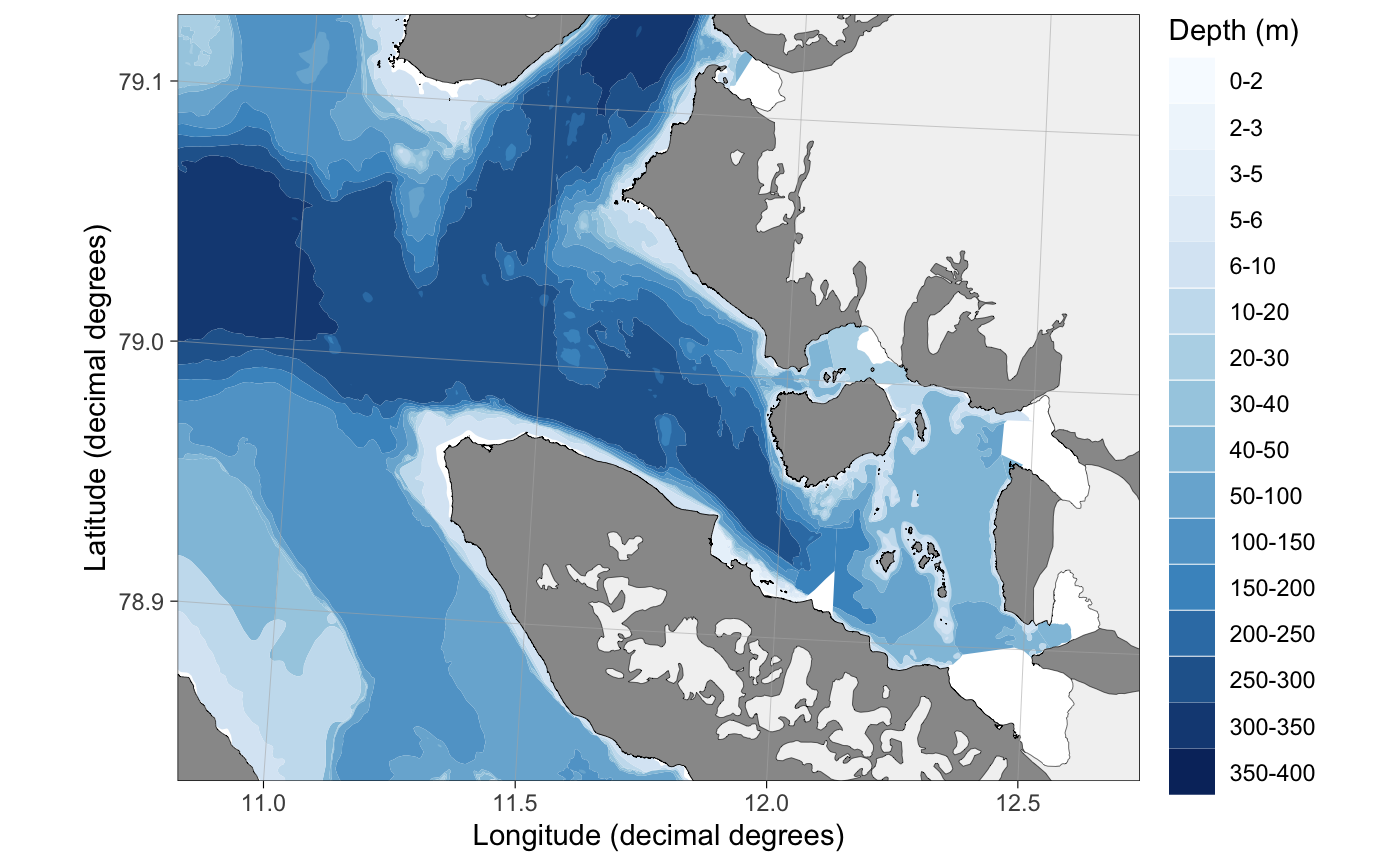
PlotSvalbard contains more detailed shapefiles from the Norwegian Mapping Authority, but these files have gaps in them. More detailed shapefiles can be plotted using the bathy.detailed argument (warning: detailed bathymetries are large and therefore slow.)
basemap("kongsfjorden", bathymetry = TRUE, bathy.detailed = TRUE)
Bathymetry styles
PlotSvalbard has 4 preprogrammed style alternatives:
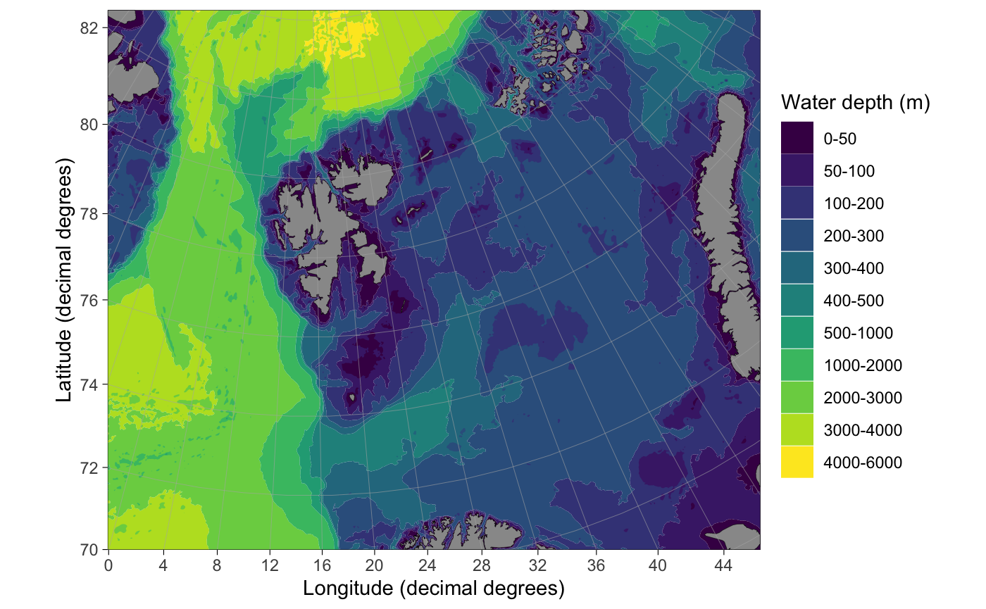
basemap("barentssea", bathymetry = TRUE, bathy.style = "poly_blues") # default

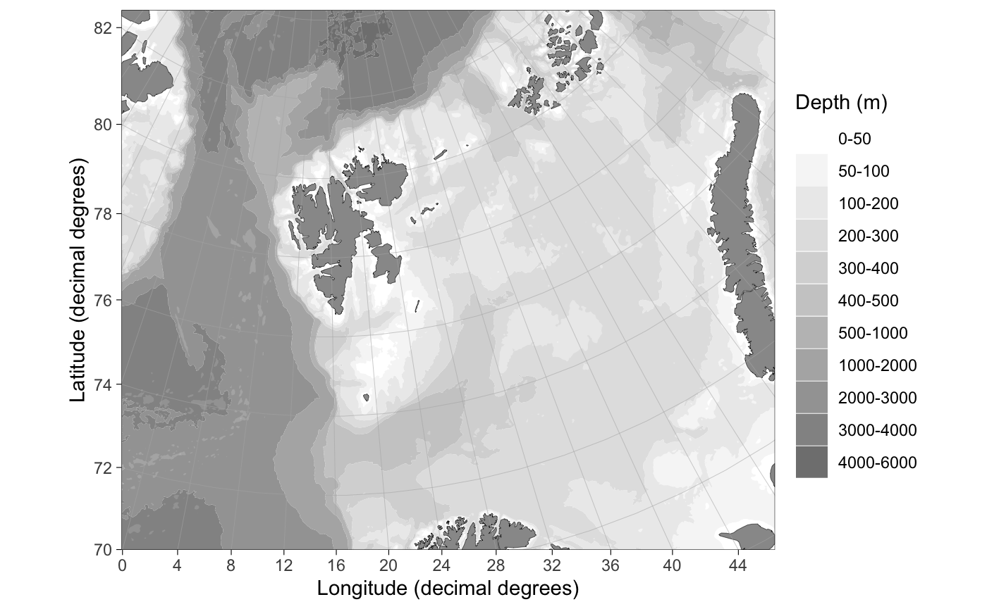
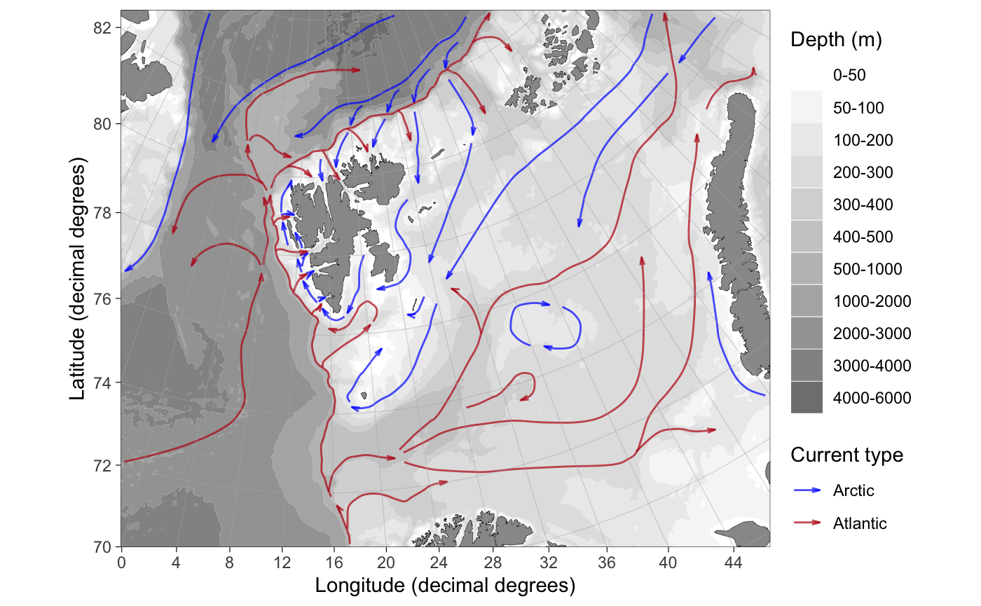
basemap("barentssea", bathymetry = TRUE, bathy.style = "poly_greys") # grey polygons with shading
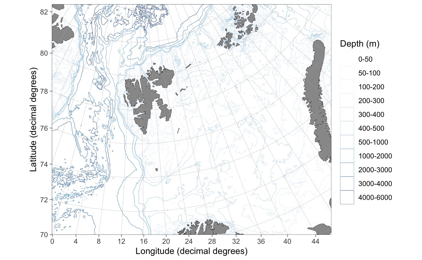
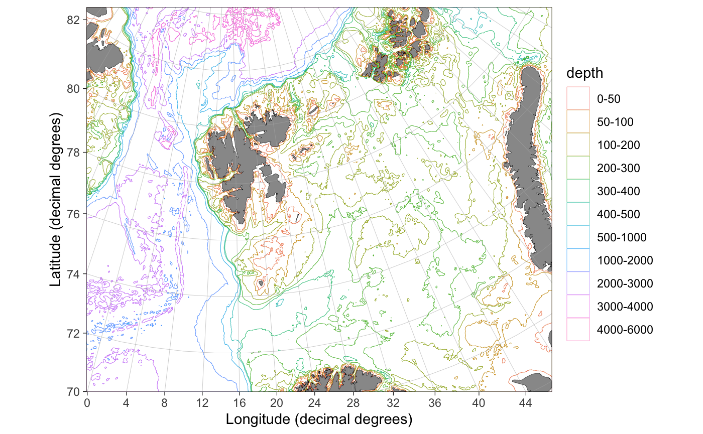
basemap("barentssea", bathymetry = TRUE, bathy.style = "contour_blues") # colored contours
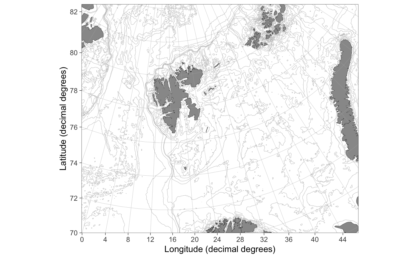
basemap("barentssea", bathymetry = TRUE, bathy.style = "contour_grey") # grey contours
Adding depth labels to contours (ala nautical maps) is currently an unresolved issue.
Ocean currents
Ocean currents for the Barents Sea have been implemented in the most recent version, but not peer-reviewed yet. This feature will be improved in the future versions of the package. Atlantic and Arctic currents are represented using red and purple arrows, respectively. The arrow color can be changed using atl.color and arc.color arguments.
basemap("barentssea", bathymetry = TRUE, bathy.style = "poly_greys", currents = TRUE, current.alpha = 0.7)
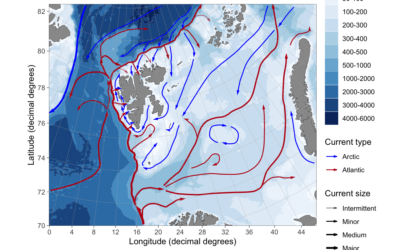
The package also supports currents, where the amount of water is approximately scaled to the thickness. The thickness is approximatation and based more on feelings than actual science
basemap("barentssea", bathymetry = TRUE, currents = TRUE, current.size = "scaled")
Adding data to basemaps
Data can be added to basemaps using the + operator and layers for ggplot2. Below you will find some examples on how to add your research data on basemaps.
Adding station labels (text)
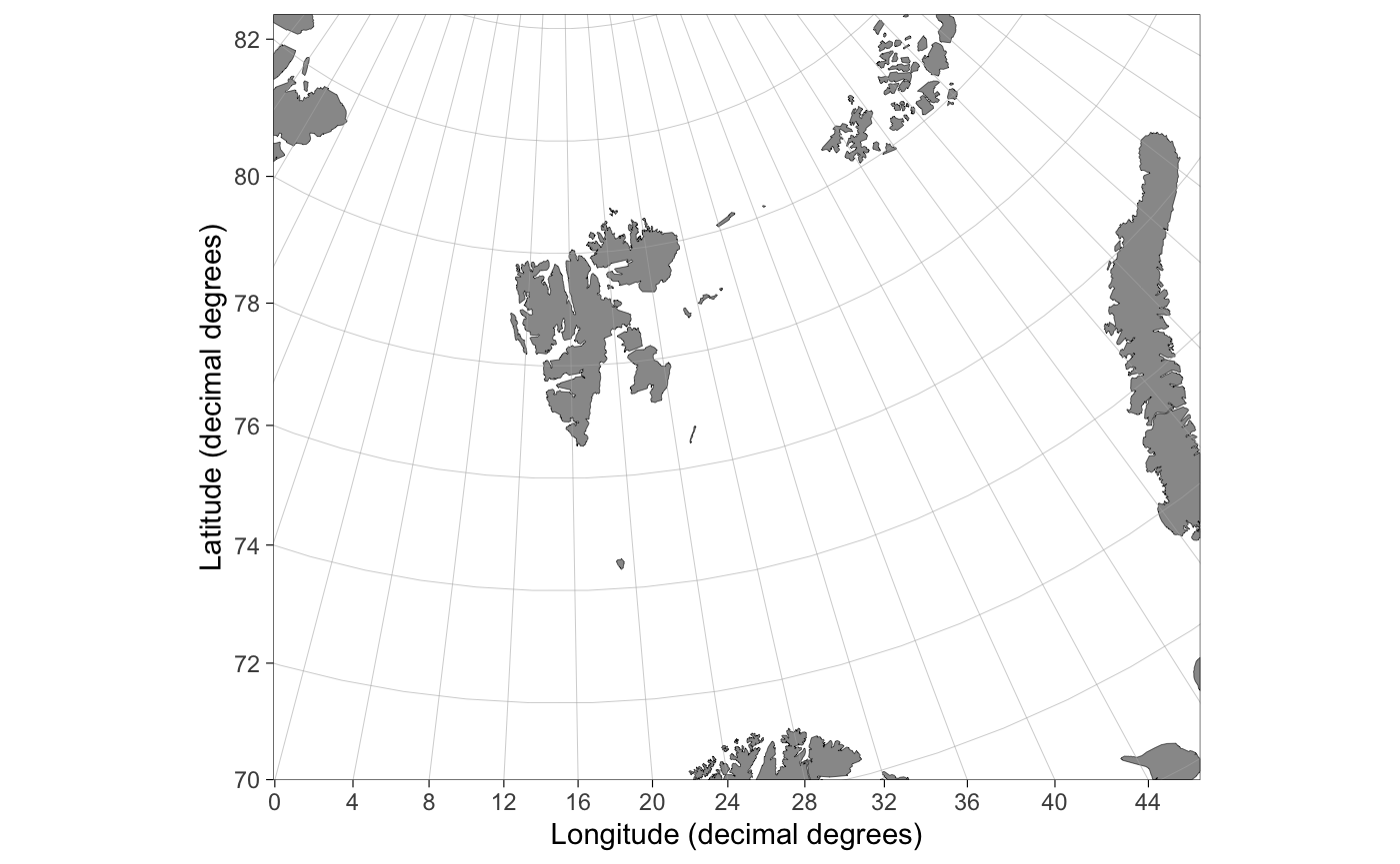
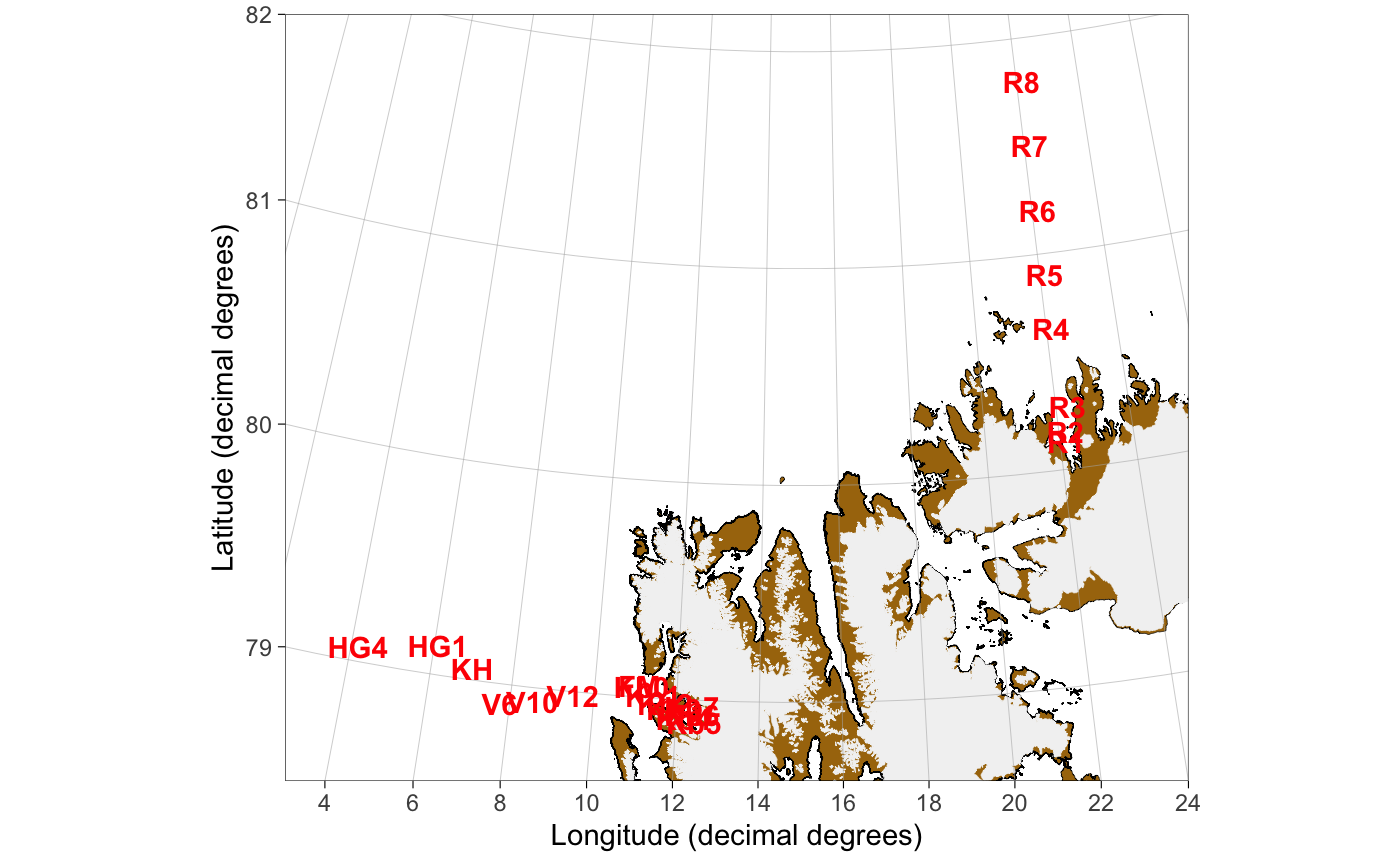
Text can be added to basemaps using the geom_text() function:
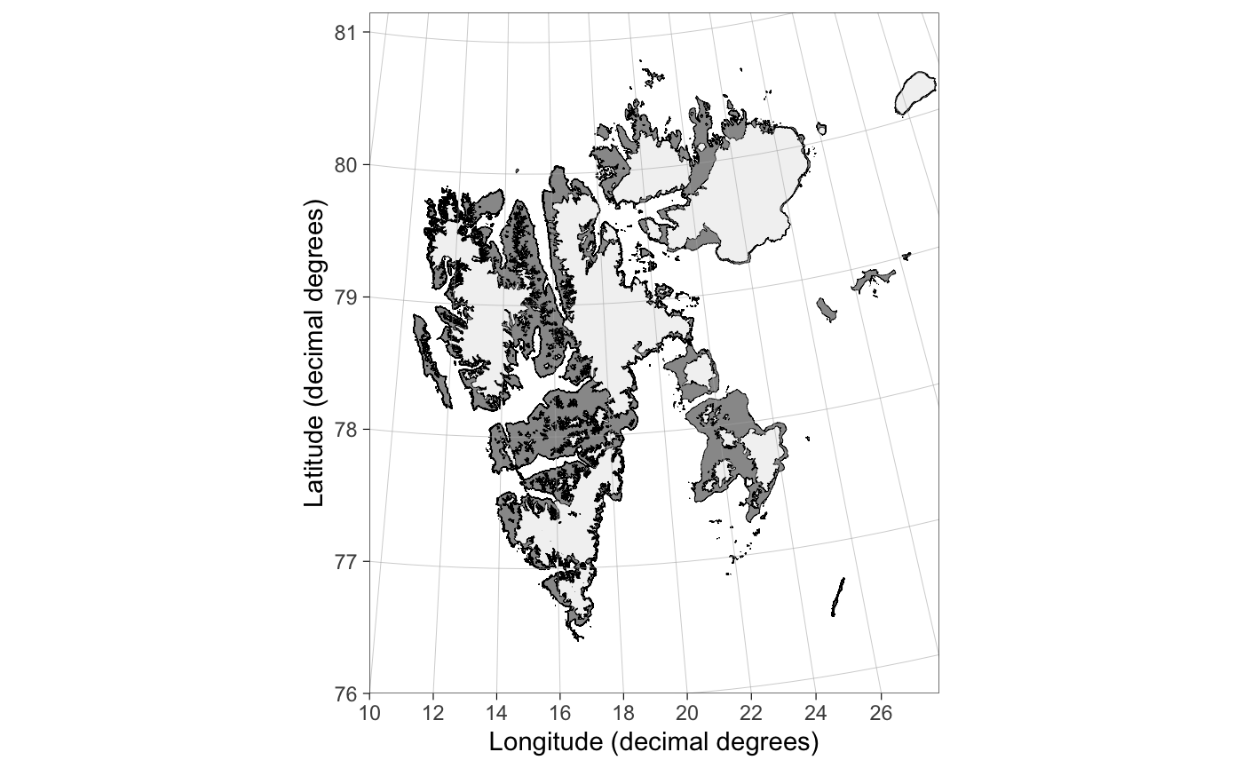
data("npi_stations")

x <- transform_coord(npi_stations, lon = "Lon", lat = "Lat", bind = TRUE)

basemap("svalbard", limits = c(3,24,78.5,82), round.lat = 1, round.lon = 2,
  land.col = "#a9750d", gla.border.col = "grey95") +
  geom_text(data = x, aes(x = lon.utm, y = lat.utm,
    label = Station), color = "red", fontface = 2)
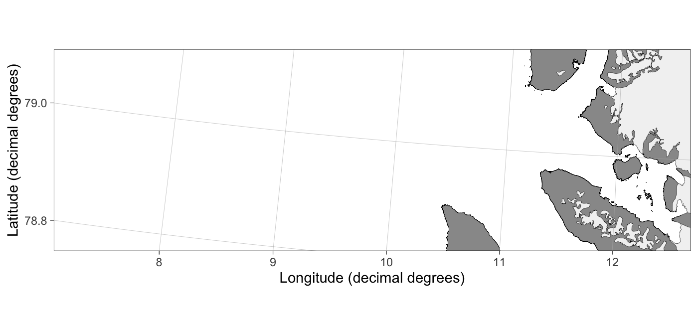
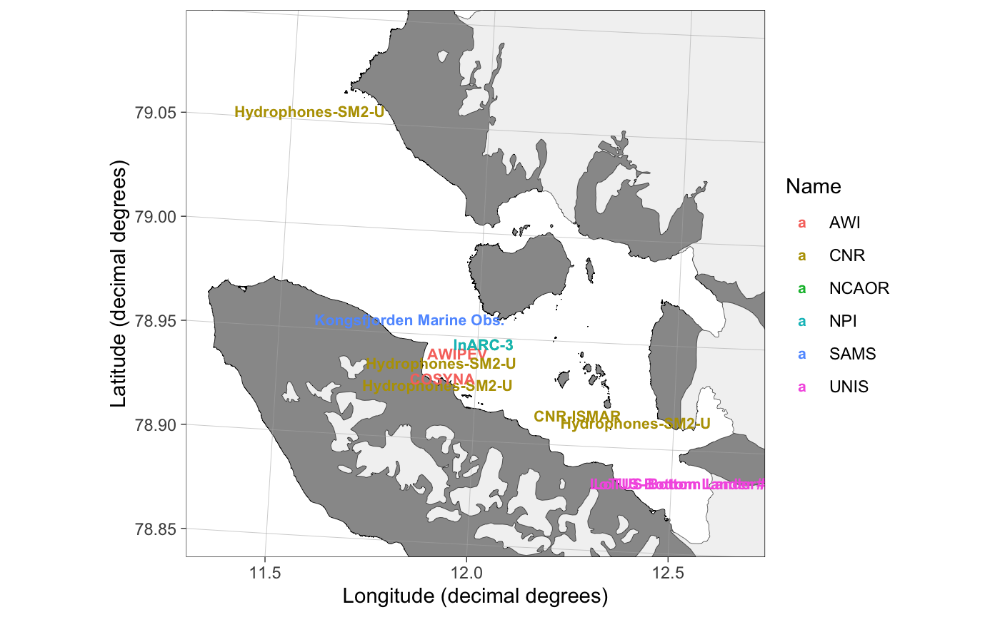
Text size can be mapped to variables using the standard ggplot2 syntax:
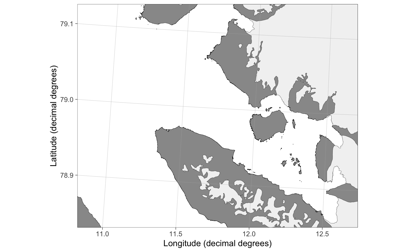
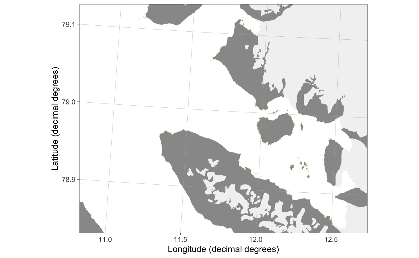
data("kongsfjord_moorings")

basemap("kongsfjorden", limits = c(11.3, 12.69, 78.85, 79.1), round.lat = 0.05, round.lon = 0.5) +
  geom_text(data = kongsfjord_moorings, aes(x = lon.utm, y = lat.utm,
  label = Mooring.name, color = Name), fontface = 2,
  size = 25.4/72.27*8) # font size = 8, see Graphical parameters
Adding piecharts
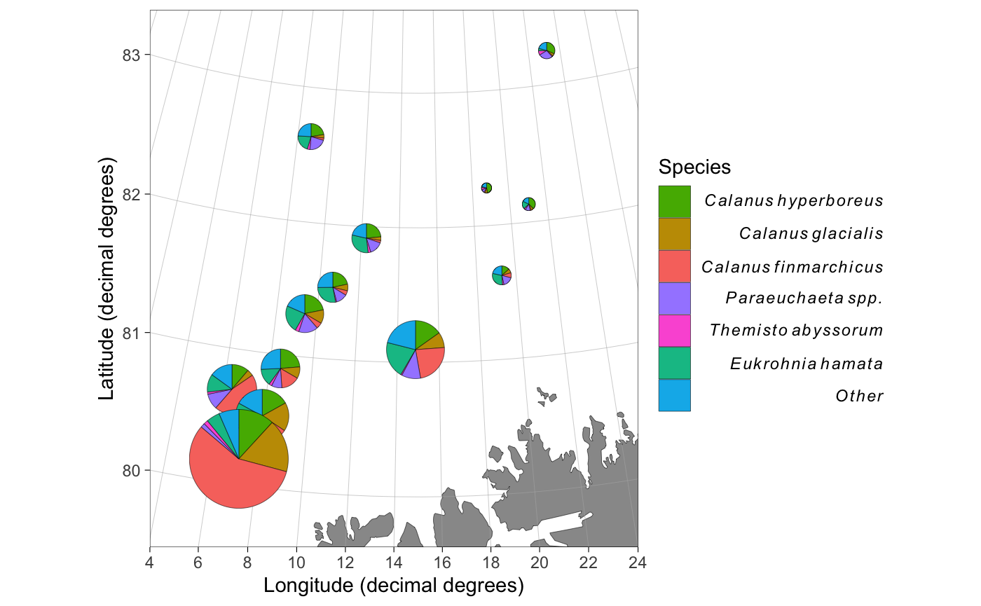
The scatterpie package allows relatively easy plotting of piecharts on maps. Extensions for ggplot2 work together with PlotSvalbard.
data(zooplankton)

x <- transform_coord(zooplankton, lon = "Longitude", lat = "Latitude", bind = TRUE)

species <- colnames(x)[!colnames(x) %in% c("lon.utm", "lat.utm", "ID",
  "Longitude", "Latitude", "Total")]

library(scatterpie)

basemap("barentssea", limits = c(4, 24, 79.5, 83.5), round.lon = 2, round.lat = 1) +
  geom_scatterpie(aes(x = lon.utm, y = lat.utm, group = ID, r = 100*Total),
  data = x, cols = species, size = 0.1) + scale_fill_discrete(name = "Species",
  breaks = species, labels = parse(text = paste0("italic(" , sub("*\\.", "~", species), ")")))
Adding interpolated 2D surfaces
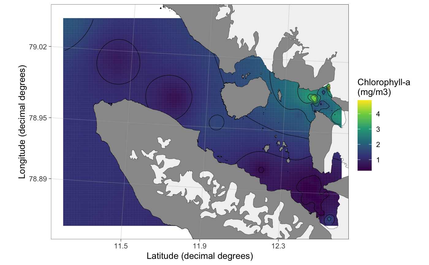
PlotSvalbard uses the krige function from the gstat package to produce interpolated 2D plots:
data("chlorophyll")

x <- interpolate_spatial(chlorophyll, Subset = "From <= 10", value = "Chla") ## Interpolate
#> [inverse distance weighted interpolation]

plot(x, legend.label = "Chlorophyll-a\n(mg/m3)")
Graphical parameters
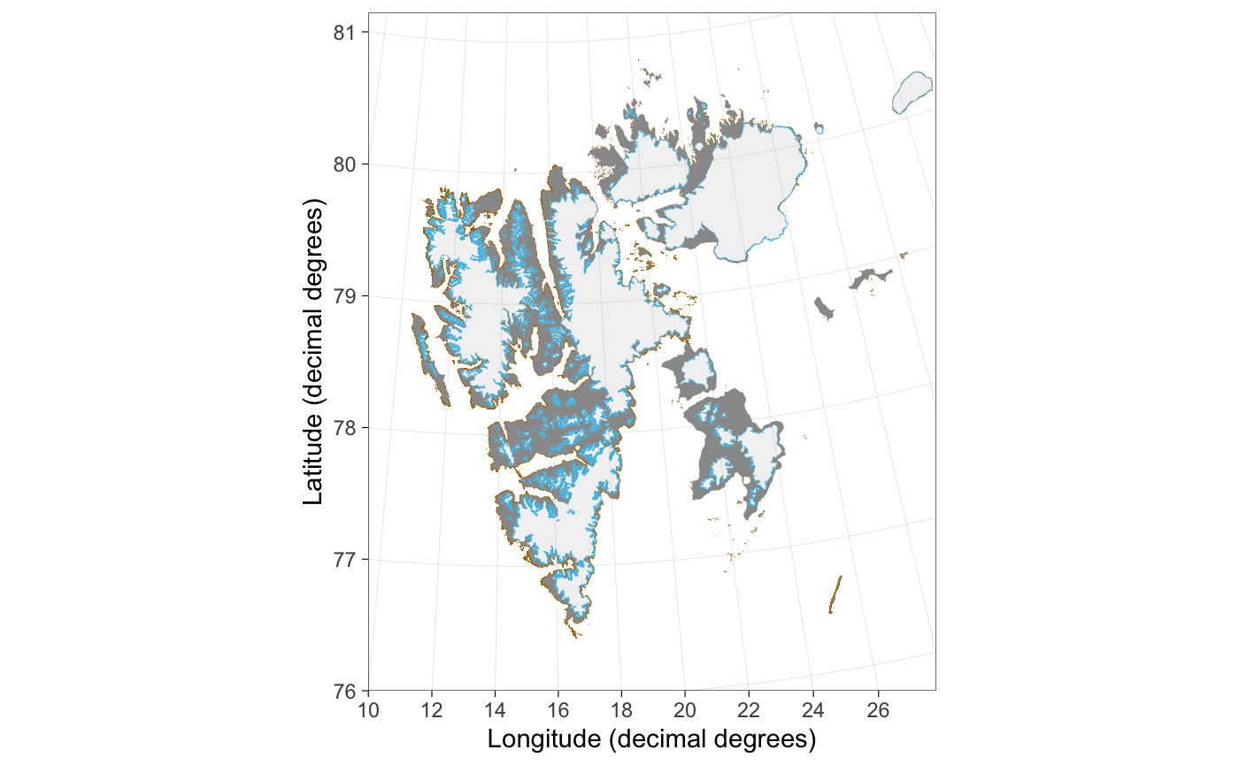
The line widths and general looks of the basemaps are optimized for a half page sized pdf figure in scientific journals (Springer figure dimensions were used to develop the function). The line widths may not look good when printed on other devices. You can modify the line widths and colors using *.size and *.border.col arguments.
basemap("svalbard", land.size = 0.01, gla.size = 0.05, grid.size = 0.05,
  gla.border.col = "#52bfe4", land.border.col = "#a9750d")
Approach to remove borders of land and glacier shapes:
basemap("kongsfjorden", gla.border.col = "grey95", land.border.col = "#eeeac4")
The line width of ggplot2 is 2.13 wider than the line widths measured as points (pt). This means that if you want a certain line width, multiply the desired line width by \(1/2.13\) inside size.* arguments. Similar conversion factor for font size is \(1/2.845276\).
The internal LS and FS functions convert line and font sizes from points to ggplot2 equivalents.
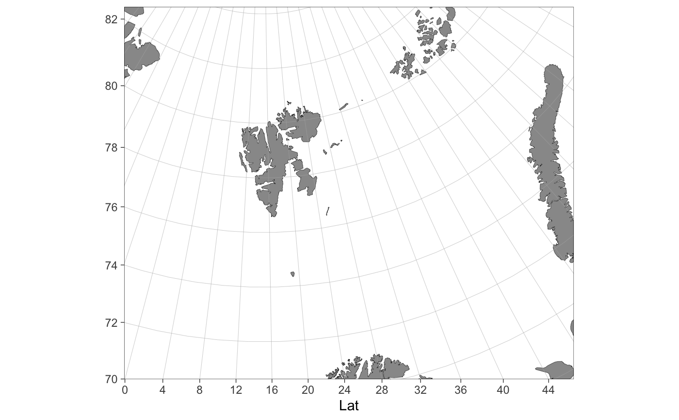
Axis labels can be modified using the labs() function family from ggplot2
basemap("barentssea") +
  labs(y = NULL) +
  xlab("Lat")
 ## Performance
The basemap("svalbard") is currently fairly slow due to less than optimized code and the large size of the shapefiles that are used to generate the map. Zoomed in maps are considerably faster than full scale Svalbard maps.
If you are looking for optimal limits for your data, you can use the basemap("barentssea") option to find these limits and replace "barentssea" with "svalbard" once you are done:
system.time(basemap("barentssea"))
#>    user  system elapsed
#>   0.406   0.021   0.443
system.time(basemap("svalbard"))
#>    user  system elapsed
#>  15.292   0.561  16.021
system.time(basemap("panarctic"))
#>    user  system elapsed
#>   1.429   0.182   1.702
system.time(basemap("barentssea", limits = c(c(19.5,23.5,80,81.7))))
#>    user  system elapsed
#>   0.145   0.007   0.157
system.time(basemap("svalbard", limits = c(c(19.5,23.5,80,81.7))))
#>    user  system elapsed
#>   3.279   0.152   3.457
system.time(basemap("panarctic", limits = c(250000, -2500000, 2000000, -250000)))
#>    user  system elapsed
#>   1.032   0.019   1.054
Oceanographic plots
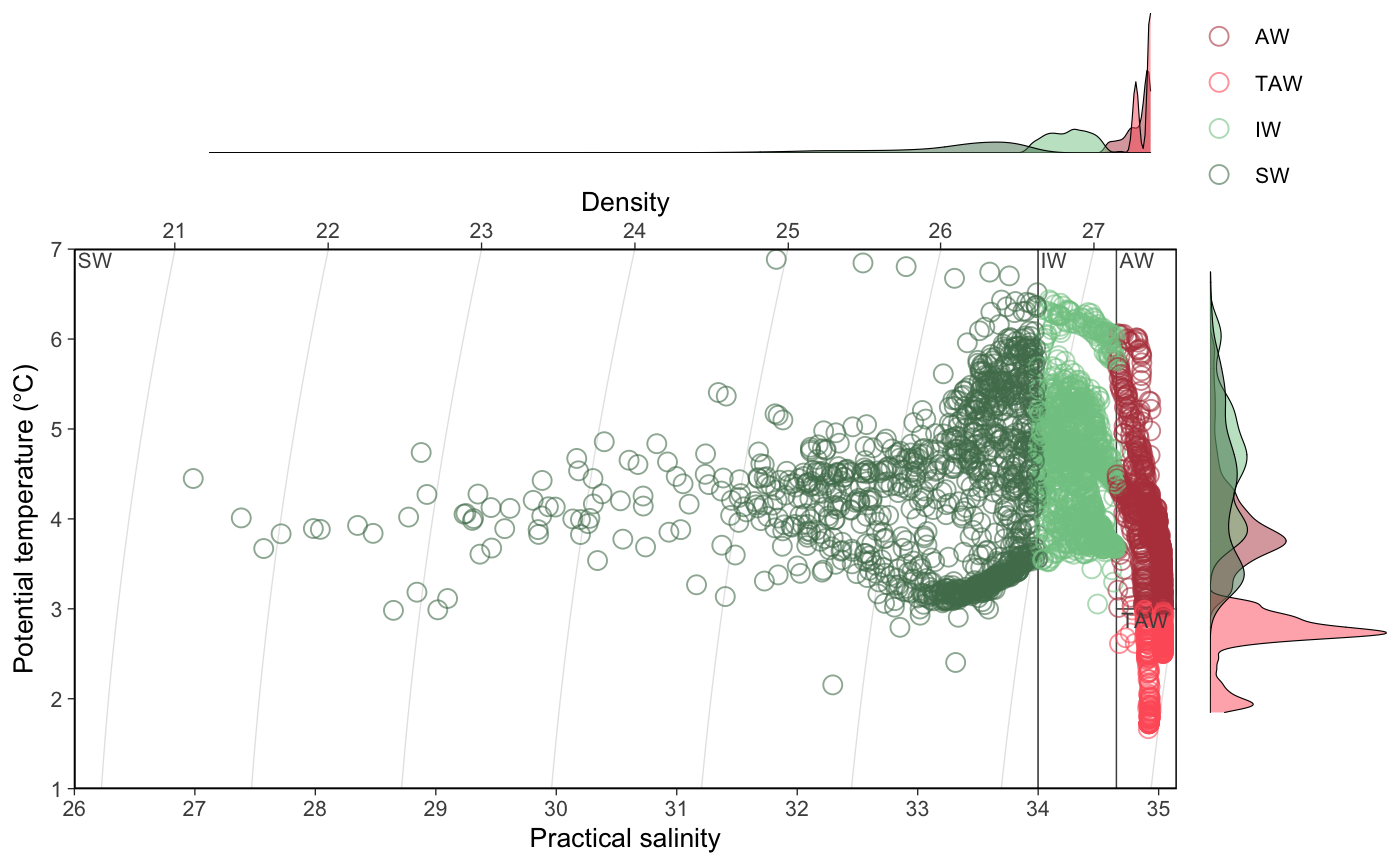
Temperature salinity plots
You can make TS-plots with water type definitions. See ?ts_plot for more plotting alternatives
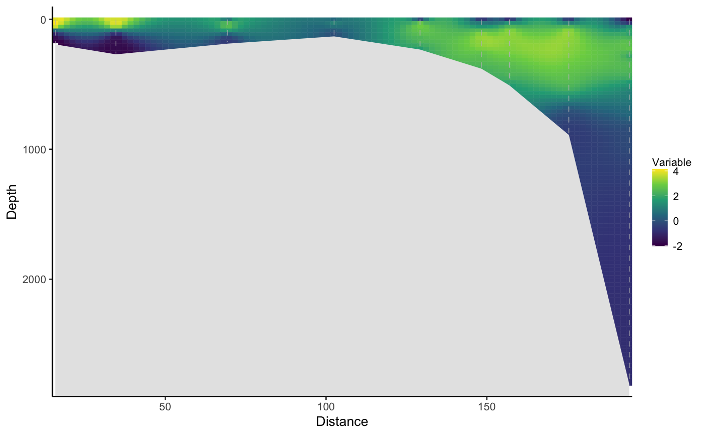
Section plots and interpolation
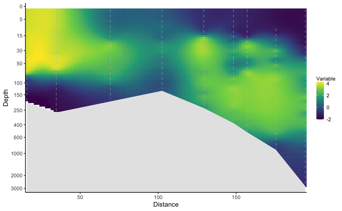
Standard temperature section plot. Difficult to see surface due to large differences in y-scale:
section_plot(ctd_rijpfjord, x = "dist", y = "pressure", z = "temp",
  bottom = "bdepth", interpolate = TRUE)
Logarithmic y axis:
section_plot(ctd_rijpfjord, x = "dist", y = "pressure", z = "temp",
  bottom = "bdepth", interpolate = TRUE, log_y = TRUE)
Contour lines:
section_plot(ctd_rijpfjord, x = "dist", y = "pressure", z = "temp",
  bottom = "bdepth", interpolate = TRUE, log_y = TRUE, contour = c(-1.8, 0, 1, 3))
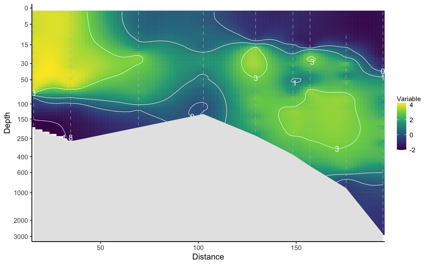
The interpolate_section function has not been documented yet here, but check the help sheet on how to use it.
Other functions
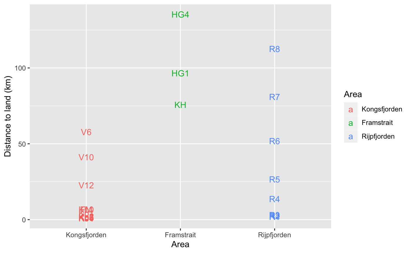
Distance to land
The dist2land function calculates the closest distance to land. Note that the function has a possibility for parallel processing, which speeds up the process with large datasets. The parallel processing has been turned off by default (cores = 1). You can turn it on by setting another integer or a function, which produces such an integer (for example parallel::detectCores() - 2 uses all avaible cores exept two). Parallelizing does not work under Windows.
library(ggplot2)
data("npi_stations")

dists <- dist2land(npi_stations, lon.col = "Lon", lat.col = "Lat", map.type = "svalbard")
dists$Area <- ordered(dists$Area, c("Kongsfjorden", "Framstrait", "Rijpfjorden"))
ggplot(dists, aes(x = Area, y = dist, label = Station, color = Area)) +
  geom_text() + ylab("Distance to land (km)") + scale_color_hue()
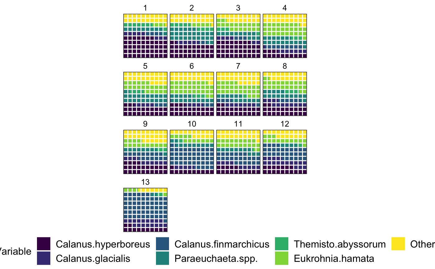
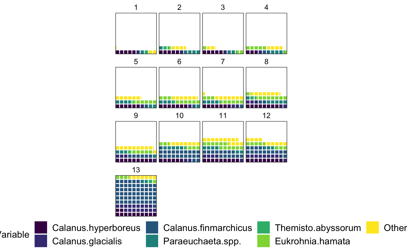
Waffle charts
Code for waffle charts has been recently implemented into the package and will be extended to enable plotting the waffles on maps. Currently the waffle plotting on maps has to be done manually using the gridand gridExtra packages (see StackOverflow how to do this). Waffle charts are filled from bottom upwards and from left to right:
library(reshape2)
data("zooplankton")

# Remove coordinates
x <- zooplankton[!names(zooplankton) %in% c("Longitude", "Latitude")]

## Make get the absolute values
x[!names(x) %in% c("ID", "Total")] <- (x[!names(x) %in% c("ID", "Total")]/100)*x$Total
x <- melt(x, id = c("ID", "Total"))

waffle_chart(x, fill = "variable", facet = "ID")
The waffles can also be scaled to maximum values
library(dplyr)

y <- x %>% group_by(ID) %>% summarise(sum = sum(value))

waffle_chart(x, fill = "variable", facet = "ID", composition = FALSE, max_value = max(y$sum))
Citing PlotSvalbard
The citation function tells how to cite PlotSvalbard package
citation("PlotSvalbard")
#>
#> To cite package 'PlotSvalbard' in publications use:
#>
#>   Mikko Vihtakari (2020). PlotSvalbard: PlotSvalbard - Plot research
#>   data from Svalbard on maps. R package version 0.9.2.
#>   https://github.com/MikkoVihtakari/PlotSvalbard
#>
#> A BibTeX entry for LaTeX users is
#>
#>   @Manual{,
#>     title = {PlotSvalbard: PlotSvalbard - Plot research data from Svalbard on maps},
#>     author = {Mikko Vihtakari},
#>     year = {2020},
#>     note = {R package version 0.9.2},
#>     url = {https://github.com/MikkoVihtakari/PlotSvalbard},
#>   }
However, please note that the maps generated by this package should be cited to their original source.
- Svalbard maps originate from the Norwegian Polar Institute. Distributed under the CC BY 4.0 license (terms of use).
- Barents Sea and pan-Arctic land shapes are downloaded from Natural Earth Data. They use the ne_10m_land and ne_50m_land (v 4.0.0) datasets, respectively. Distributed under the CC Public Domain license (terms of use).
- Pan-Arctic bathymetry shapefile is generalized from General Bathymetric Chart of the Oceans One Minute Grid.
- Barents Sea bathymetry shapefile is generalized from IBCAO v3.0 500m RR grid. Should be cited as Jakobsson, M., et al. The International Bathymetric Chart of the Arctic Ocean (IBCAO) Version 3.0. Geophys. Res. Lett. 2012, 39:L12609.
- Svalbard fjord bathymetry shapefiles are from the Norwegian Mapping Authority. Distributed under the CC BY 4.0 license.
The example data included in the package are property of the Norwegian Polar Institute and should not be used in other instances. I.e. these data are unpublihed at the moment.