Calculates the closest distance to land within a map type for a given set of coordinates
dist2land(
  x,
  lon.col = NULL,
  lat.col = NULL,
  map.type = "panarctic",
  bind = TRUE,
  dist.col = "dist",
  return.binary = FALSE,
  geodesic.distances = FALSE,
  cores = 1
)
Arguments
| x | Data.frame containing geographic coordinates as decimal degrees |
|---|---|
| lon.col | The name of the longitude column in |
| lat.col | The name of the latitude column in |
| map.type | a character string specifying the map type which land boundaries should be used for the distance calculation. See the |
| bind | Logical indicating whether |
| dist.col | The name of the distance column, if |
| return.binary | Logical indicating whether binary (TRUE = the position is in the ocean, FALSE = the position is on land) should be returned instead of distances. Speeds up the function considerably. |
| geodesic.distances | Logical indicating whether |
| cores | Integer value defining how many cores should be used in the calculations. Parallelization speeds up the function (see |
Value
If bind = TRUE, returns a data frame with calculated distances to land. If bind = FALSE returns vector in the same order than coordinates specified in x. Distances are returned as kilometers. If return_binary = TRUE, binary values are returned instead of distances (TRUE = the position is in the ocean, FALSE = the position is on land).
Details
If geodesic.distances = FALSE, the function uses the gDistance function to calculate closest distances between coordinates in x and a specified SpatialPolygonsDataframe object. The spatial object (map) can be specified using the map.type argument. If geodesic.distances = TRUE, the dist2Line is used to calculate similar distances assumming an elliptical Earth. The dist2Line function is presumably more exact, especially for pan-Arctic maps, but considerably slower.
The function is very slow for large datasets. If you only want to use the function to remove (wrong) observations reported on land, set the return.binary argument to TRUE. This speeds up the function considerably.
The function has a possibility for parallel processing, which speeds up the calculations for large datasets. The parallel processing has been turned off by default (cores = 1). You can turn it on by setting another integer or a function, which produces such an integer (for example parallel::detectCores() - 2 uses all avaible cores exept two). Parallelizing does not work under Windows.
Examples
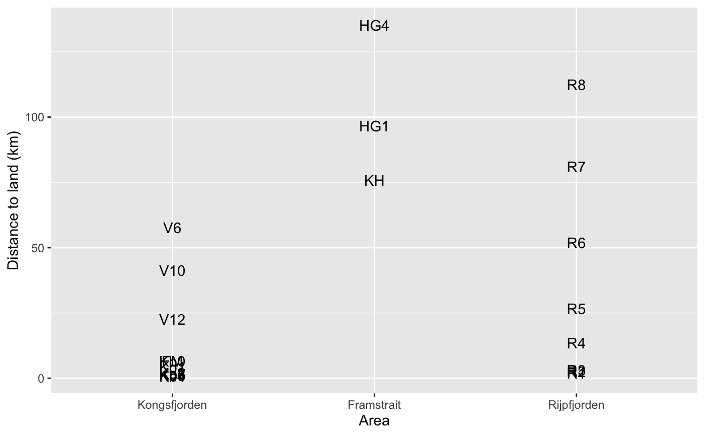
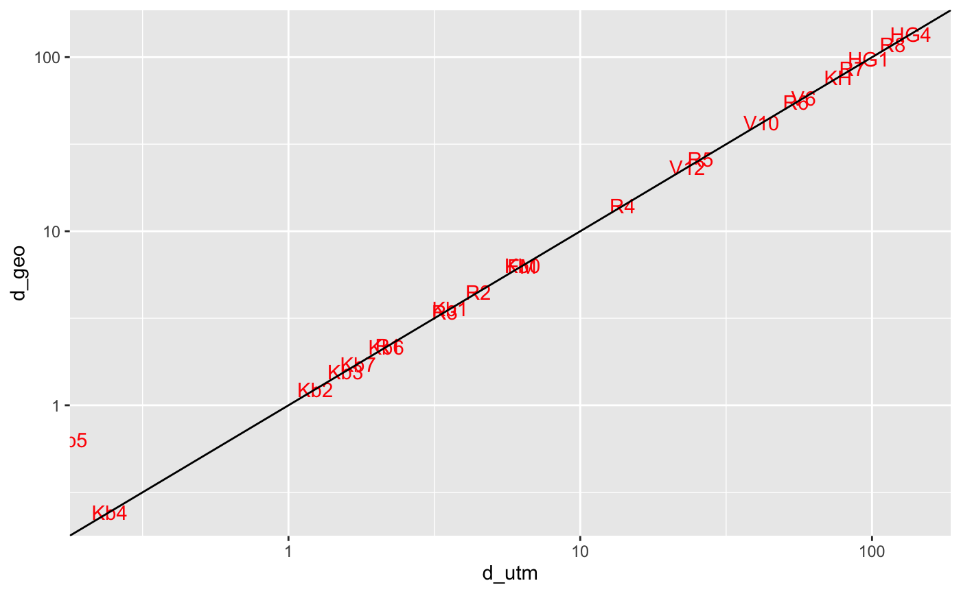
## Distances from land using UTM coordinates library(ggplot2) data("npi_stations") dists <- dist2land(npi_stations, map.type = "svalbard")#> | | | 0% | |=== | 4% | |====== | 9% | |========= | 13% | |============ | 17% | |=============== | 22% | |================== | 26% | |===================== | 30% | |======================== | 35% | |=========================== | 39% | |============================== | 43% | |================================= | 48% | |===================================== | 52% | |======================================== | 57% | |=========================================== | 61% | |============================================== | 65% | |================================================= | 70% | |==================================================== | 74% | |======================================================= | 78% | |========================================================== | 83% | |============================================================= | 87% | |================================================================ | 91% | |=================================================================== | 96% | |======================================================================| 100%dists$Area <- ordered(dists$Area, c("Kongsfjorden", "Framstrait", "Rijpfjorden")) ggplot(dists, aes(x = Area, y = dist, label = Station)) + geom_text() + ylab("Distance to land (km)")## Geodesic distances are presumably more exact, ## but much slower to calculate. Do not use detailed ## maps for these: d_utm <- dist2land(npi_stations, map.type = "barentssea", dist.col = "d_utm")#> | | | 0% | |=== | 4% | |====== | 9% | |========= | 13% | |============ | 17% | |=============== | 22% | |================== | 26% | |===================== | 30% | |======================== | 35% | |=========================== | 39% | |============================== | 43% | |================================= | 48% | |===================================== | 52% | |======================================== | 57% | |=========================================== | 61% | |============================================== | 65% | |================================================= | 70% | |==================================================== | 74% | |======================================================= | 78% | |========================================================== | 83% | |============================================================= | 87% | |================================================================ | 91% | |=================================================================== | 96% | |======================================================================| 100%d_geo <- dist2land(npi_stations, map.type = "barentssea", geodesic.distances = TRUE, dist.col = "d_geo") y <- merge(d_utm[c("Station", "d_utm")], d_geo[c("Station", "d_geo")]) ggplot(y, aes(x = d_utm, y = d_geo, label = Station)) + geom_text(color = "red") + geom_abline(slope=1, intercept=0) + scale_x_log10() + scale_y_log10()#> Warning: Transformation introduced infinite values in continuous x-axis## The processing time difference between binary, geodesic and UTM distances: # Binary: system.time(dist2land(npi_stations, map.type = "barentssea", return.binary = TRUE))#> user system elapsed #> 0.022 0.001 0.027#> user system elapsed #> 0.017 0.000 0.017 # UTM: system.time(dist2land(npi_stations, map.type = "barentssea"))#> | | | 0% | |=== | 4% | |====== | 9% | |========= | 13% | |============ | 17% | |=============== | 22% | |================== | 26% | |===================== | 30% | |======================== | 35% | |=========================== | 39% | |============================== | 43% | |================================= | 48% | |===================================== | 52% | |======================================== | 57% | |=========================================== | 61% | |============================================== | 65% | |================================================= | 70% | |==================================================== | 74% | |======================================================= | 78% | |========================================================== | 83% | |============================================================= | 87% | |================================================================ | 91% | |=================================================================== | 96% | |======================================================================| 100%#> user system elapsed #> 0.068 0.001 0.069#> user system elapsed #> 0.073 0.003 0.073 # Geodesic: system.time(dist2land(npi_stations, map.type = "barentssea", geodesic.distances = TRUE))#> user system elapsed #> 15.521 0.847 16.400#> user system elapsed #> 14.096 0.615 14.755 ## Despite the inaccuracy due to polar stereographic protection ## the UTM version seems to produce feasible distances from land ## on pan-Arctic scale data("meiofauna") d_panarctic <- dist2land(meiofauna, lon.col = "Lon", lat.col = "Lat", map.type = "panarctic")#> | | | 0% | | | 1% | |= | 1% | |= | 2% | |== | 2% | |== | 3% | |== | 4% | |=== | 4% | |=== | 5% | |==== | 5% | |==== | 6% | |===== | 7% | |===== | 8% | |====== | 8% | |====== | 9% | |======= | 9% | |======= | 10% | |======= | 11% | |======== | 11% | |======== | 12% | |========= | 12% | |========= | 13% | |========= | 14% | |========== | 14% | |========== | 15% | |=========== | 15% | |=========== | 16% | |============ | 17% | |============ | 18% | |============= | 18% | |============= | 19% | |============== | 19% | |============== | 20% | |============== | 21% | |=============== | 21% | |=============== | 22% | |================ | 22% | |================ | 23% | |================= | 24% | |================= | 25% | |================== | 25% | |================== | 26% | |=================== | 26% | |=================== | 27% | |=================== | 28% | |==================== | 28% | |==================== | 29% | |===================== | 29% | |===================== | 30% | |===================== | 31% | |====================== | 31% | |====================== | 32% | |======================= | 32% | |======================= | 33% | |======================= | 34% | |======================== | 34% | |======================== | 35% | |========================= | 35% | |========================= | 36% | |========================== | 36% | |========================== | 37% | |========================== | 38% | |=========================== | 38% | |=========================== | 39% | |============================ | 39% | |============================ | 40% | |============================ | 41% | |============================= | 41% | |============================= | 42% | |============================== | 42% | |============================== | 43% | |============================== | 44% | |=============================== | 44% | |=============================== | 45% | |================================ | 45% | |================================ | 46% | |================================= | 47% | |================================= | 48% | |================================== | 48% | |================================== | 49% | |=================================== | 49% | |=================================== | 50% | |=================================== | 51% | |==================================== | 51% | |==================================== | 52% | |===================================== | 52% | |===================================== | 53% | |====================================== | 54% | |====================================== | 55% | |======================================= | 55% | |======================================= | 56% | |======================================== | 56% | |======================================== | 57% | |======================================== | 58% | |========================================= | 58% | |========================================= | 59% | |========================================== | 59% | |========================================== | 60% | |========================================== | 61% | |=========================================== | 61% | |=========================================== | 62% | |============================================ | 62% | |============================================ | 63% | |============================================ | 64% | |============================================= | 64% | |============================================= | 65% | |============================================== | 65% | |============================================== | 66% | |=============================================== | 66% | |=============================================== | 67% | |=============================================== | 68% | |================================================ | 68% | |================================================ | 69% | |================================================= | 69% | |================================================= | 70% | |================================================= | 71% | |================================================== | 71% | |================================================== | 72% | |=================================================== | 72% | |=================================================== | 73% | |=================================================== | 74% | |==================================================== | 74% | |==================================================== | 75% | |===================================================== | 75% | |===================================================== | 76% | |====================================================== | 77% | |====================================================== | 78% | |======================================================= | 78% | |======================================================= | 79% | |======================================================== | 79% | |======================================================== | 80% | |======================================================== | 81% | |========================================================= | 81% | |========================================================= | 82% | |========================================================== | 82% | |========================================================== | 83% | |=========================================================== | 84% | |=========================================================== | 85% | |============================================================ | 85% | |============================================================ | 86% | |============================================================= | 86% | |============================================================= | 87% | |============================================================= | 88% | |============================================================== | 88% | |============================================================== | 89% | |=============================================================== | 89% | |=============================================================== | 90% | |=============================================================== | 91% | |================================================================ | 91% | |================================================================ | 92% | |================================================================= | 92% | |================================================================= | 93% | |================================================================== | 94% | |================================================================== | 95% | |=================================================================== | 95% | |=================================================================== | 96% | |==================================================================== | 96% | |==================================================================== | 97% | |==================================================================== | 98% | |===================================================================== | 98% | |===================================================================== | 99% | |======================================================================| 99% | |======================================================================| 100%d_panarctic <- transform_coord(d_panarctic, lon = "Lon", lat = "Lat", map.type = "panarctic", bind = TRUE) basemap("panarctic", limits = c("d_panarctic", "lon.utm", "lat.utm")) + geom_point(data = d_panarctic, aes(x = lon.utm, y = lat.utm, color = dist), size = 3) + scale_color_viridis_c(name = "Distance (km)")#> Error in get(limits[1]): object 'd_panarctic' not found

